

How to Make a Table in Excel


In this tutorial, you will learn how to make a table in excel completely. We will also discuss the ways to use a table to optimally manage and process your data.
The table can be a crucial feature to use when you work in excel. If you want to organize your data much better, then you should know how to apply tables to them effectively.
Want to understand more about the excel table feature? We will discuss all the things you need to know here!
Disclaimer: This post may contain affiliate links from which we earn commission from qualifying purchases/actions at no additional cost for you. Learn more
Want to work faster and easier in Excel? Install and use Excel add-ins! Read this article to know the best Excel add-ins to use according to us!
Table of Contents:
- What is an excel table?
- Excel table functions
- Types of tables in excel
- An excel table example
- How to make a table in excel: the step-by-step
- Why my table doesn’t expand for new data?
- How to sort and filter data in an excel table
- How to get numbers total in an excel table
- Formulas in an excel table
- How to name/rename a table in excel
- How to refer to table columns in an excel formula
- How to print only your excel table from your worksheet (only for Windows)
- How to move a table in excel
- How to use table styles to change a table interface in excel (how to color a table in excel)
- How to make and thicken a table border line in excel
- How to increase/reduce a table size in excel
- How to join/combine tables in excel
- How to lock a table in excel
- How to remove a table formatting in excel
- How to remove a table in excel
- Exercise
- Additional note
What is an Excel Table?
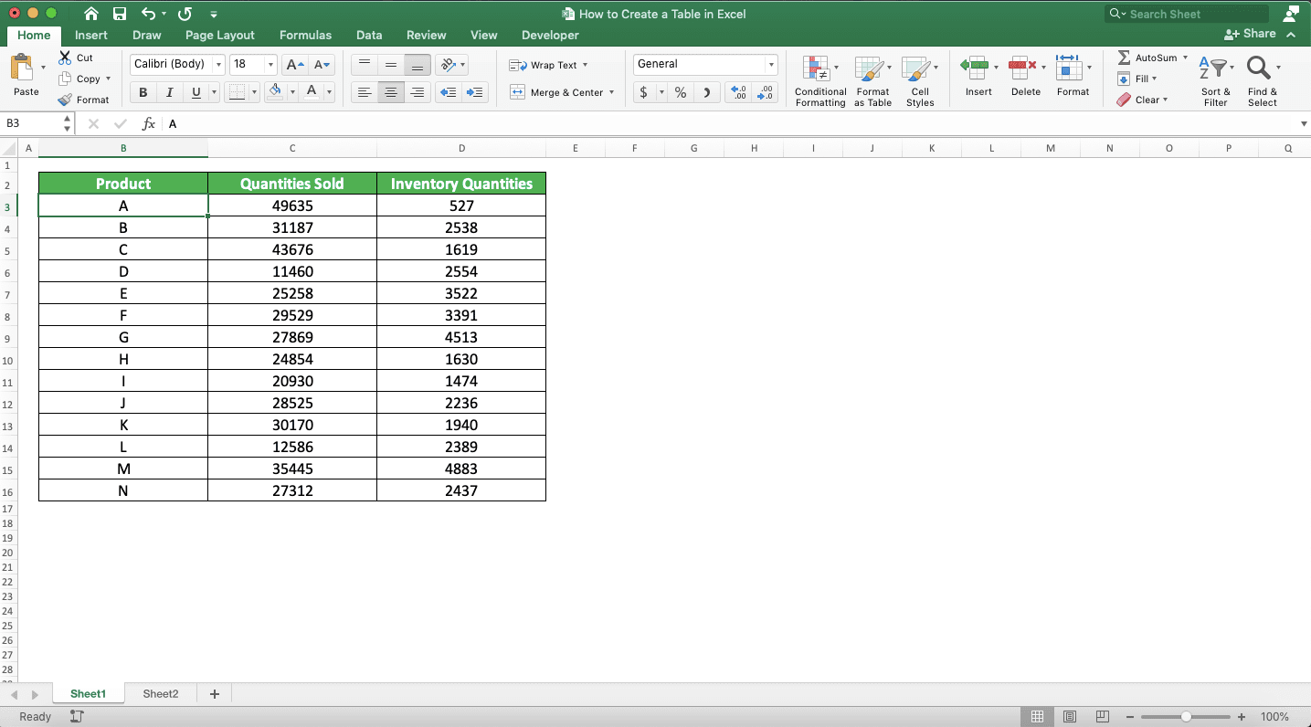
Excel table is an Excel feature that creates a distinct group for the data in a cell range. We can run some special functions exclusively on those data we group in the table.You can see what an excel table looks like in excel in the screenshot below.
Excel Table Functions
By using a table in excel, we can:- Display a clear distinction between a group of data and other data outside the group
- Process our selected group of data much faster with some special features
- Refer to parts of our table easily when we write a formula
Types of Tables in Excel
Generally, there are three types of tables we can use in excel. The table we make using the excel table feature is one of them.Here are those three table types with a bit of their explanation.
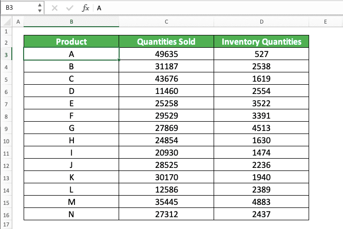
- Simple table (or “gray cell” table): the table we create normally in a cell range (without applying the excel table feature)
- Excel table: the table we create using the excel table feature. We usually use it to group data exclusively and run some special functions for the data in the group only
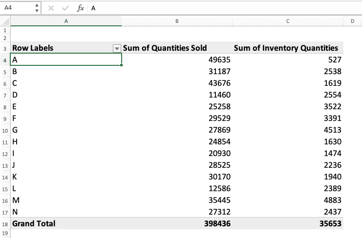
- Pivot table: the table we create using the excel pivot table feature. We usually use it to organize, analyze, and get insights from the data that we have fast
In this tutorial, we will focus to discuss the table we create using the excel table feature. That is because this is the table most people refer to when they talk about creating a table in excel.
For a better understanding of the excel table types, see the examples of simple table and pivot table below.
Simple table
Pivot table
An Excel Table Example
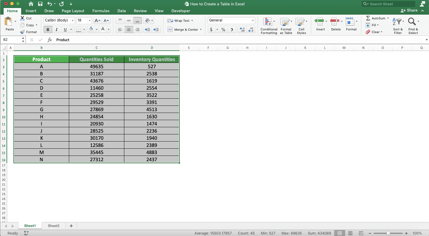
Let’s take a look again at the excel table example we saw much earlier.
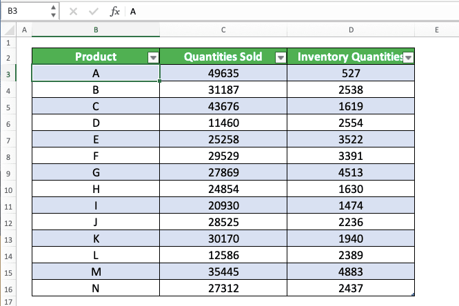
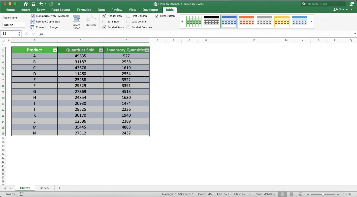
When you apply the table feature to a cell range, Excel will apply different colors for even and odd rows. Sort & filter buttons will also show up on your table headers as you can see in the screenshot.
When the cell range is already in a table form, we can utilize special features for the table data. We can sort, filter, remove duplicates, add slicers, and form a pivot table among others. We can also change the table template and run formulas to process the table data fast.
Furthermore, we can name the table using the name we want. When we want to refer to the data in the table, we can use the table name to do it.
When we input data to the columns or rows just outside the table, it will expand itself to include them.
How to Make a Table in Excel: the Step-by-Step
Want to know how to apply the table feature to a cell range? Here are the simple yet detailed steps to do it.-
Prepare the cell range you want to convert into a table. You should already separate the data into columns and rows and it is better if there are headers
-
Highlight the cell range you want to make a table of
-
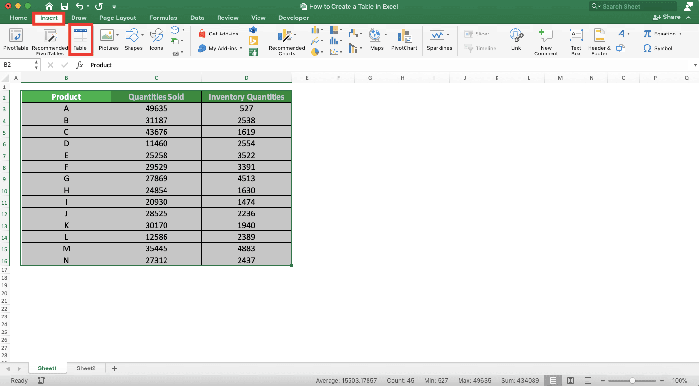
Go to the Insert tab and click the Table button
-
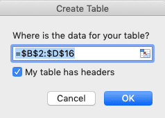
Make sure your cell range is already in the text box of the dialog box that shows up. Check/uncheck the “My table has headers” checkbox depending on whether your cell range has headers or not
-
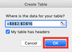
Click Enter
-
Done!
Why My Table Doesn’t Expand for New Data?
By default, the excel table automatically expands itself whenever there is data you input just right or below it.If your table doesn’t do that, then you might have changed the default settings without knowing. If you want, you can turn back the default setting by doing these following steps.
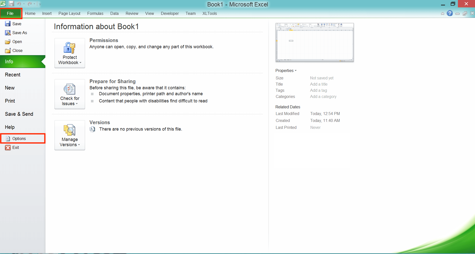
First, click File and then Options (For Mac, click Excel and then Preferences…).
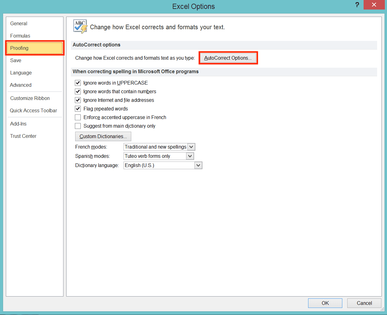
In the dialog box that shows up, choose Proofing on the left side. Then, click the AutoCorrect Options button in the Proofing menu on the right (click Table & Filters button in Mac)
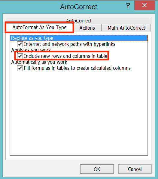
In another dialog box that shows up, go to the AutoFormat as You Type tab. Make sure you check the Include new rows and columns in table checkbox (In Mac, check the Automatically expand tables checkbox).
Then, click OK and OK. Now, your table should automatically expand itself whenever you input new entries just outside your table!
How to Sort and Filter Data in an Excel Table
As you usually get sort & filter buttons in your table headers immediately after you create a table, this should be easy.Just click the sort & filter button on the header you want as the reference of your sort & filter process. Then, choose the action you want to do from the choices that show up.
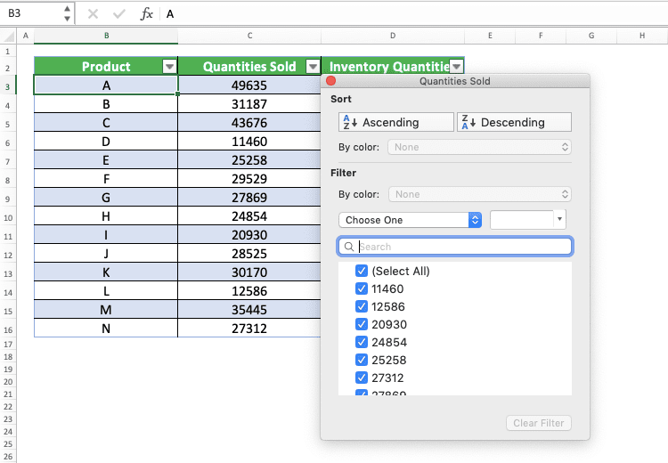
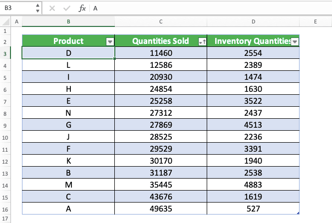
The table will display its data based on the action choice you take. In the example, we sort the table based on the ascending order of the quantities sold column.
How to Get Numbers Total in an Excel Table
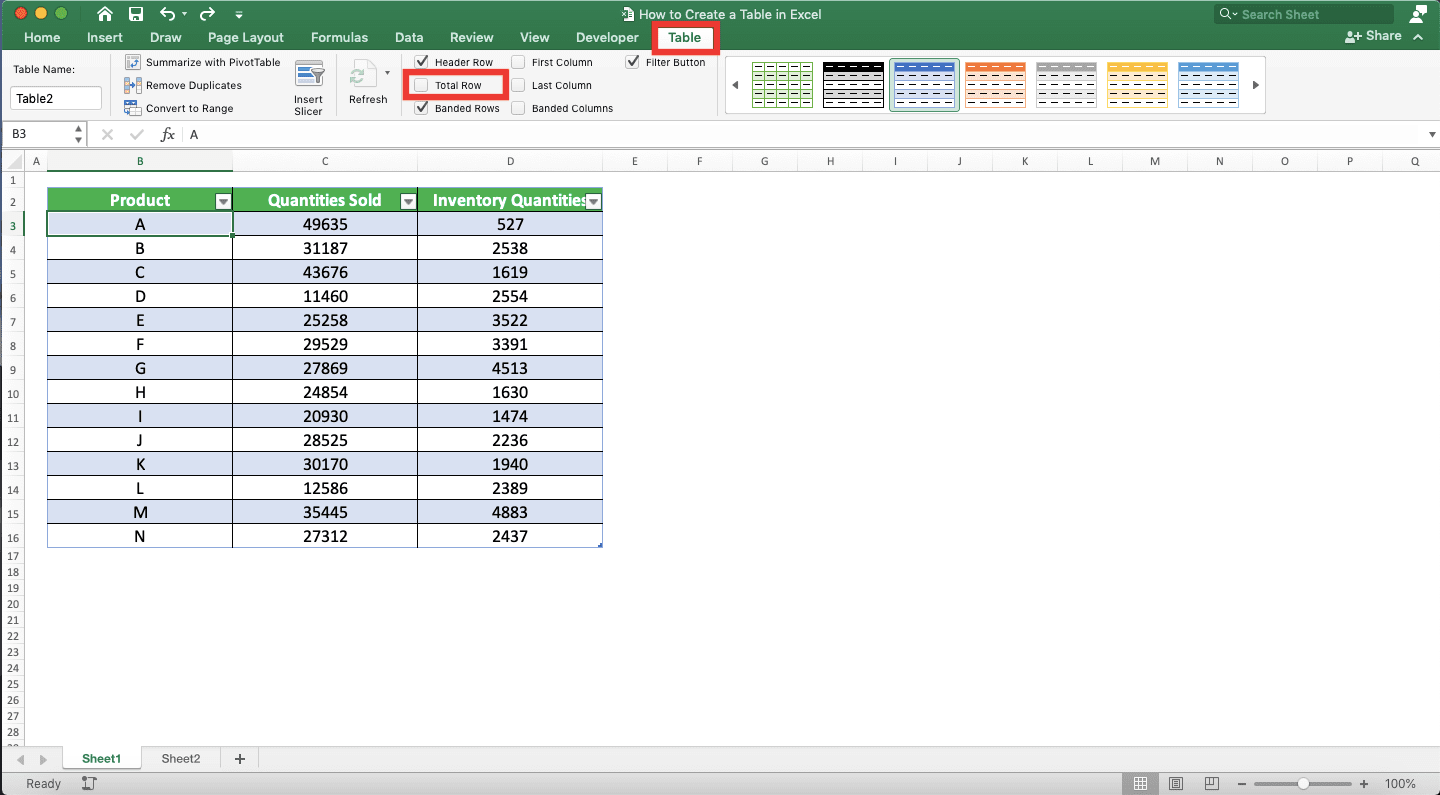
Need to get the total of the numbers in your table’s column? It is an easy thing to do with the feature that the excel table has.Just activate the total row feature in your table. Put your cell cursor anywhere in the table and go to the Table tab in the excel ribbon. Then, check the Total Row checkbox inside the tab.
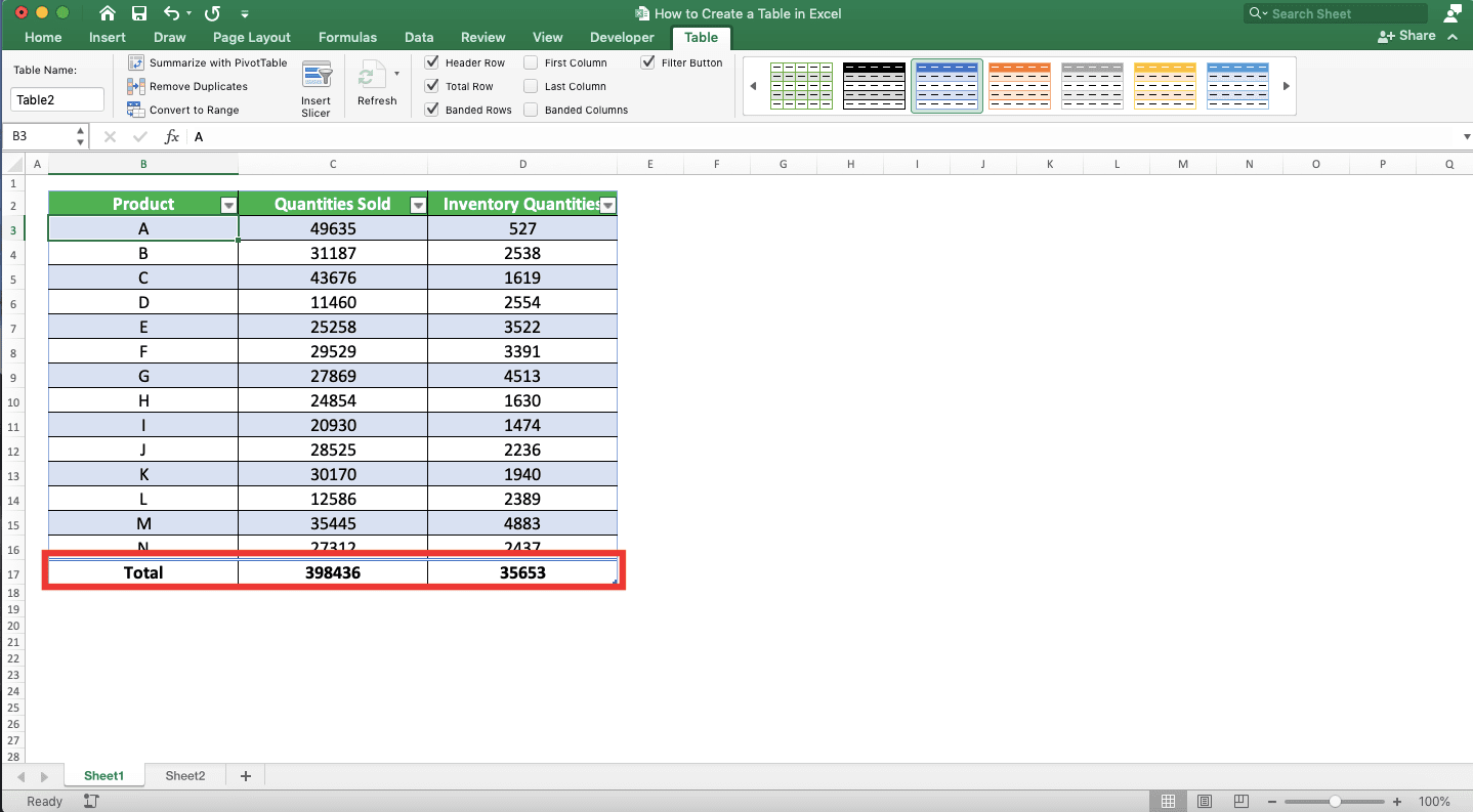
Excel will immediately add a row that sums your numbers per column!
Formulas in an Excel Table
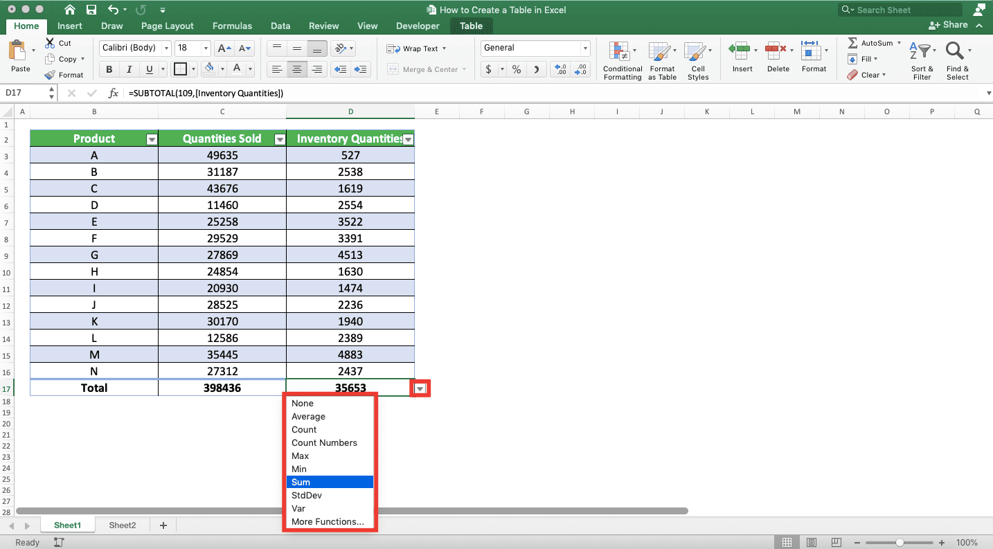
If you want to process the data in your table columns, you can do it easier with the total row feature. Besides sum, the total row can also average, count, and apply other formulas to the data per column.Just place your cell cursor in the total row cell in the column which data you want to process. Then, click the dropdown and choose the formula you want to apply.
If you want to apply a formula to the table data per row fast, then you can do this. Type the formula in the column just next to the table.
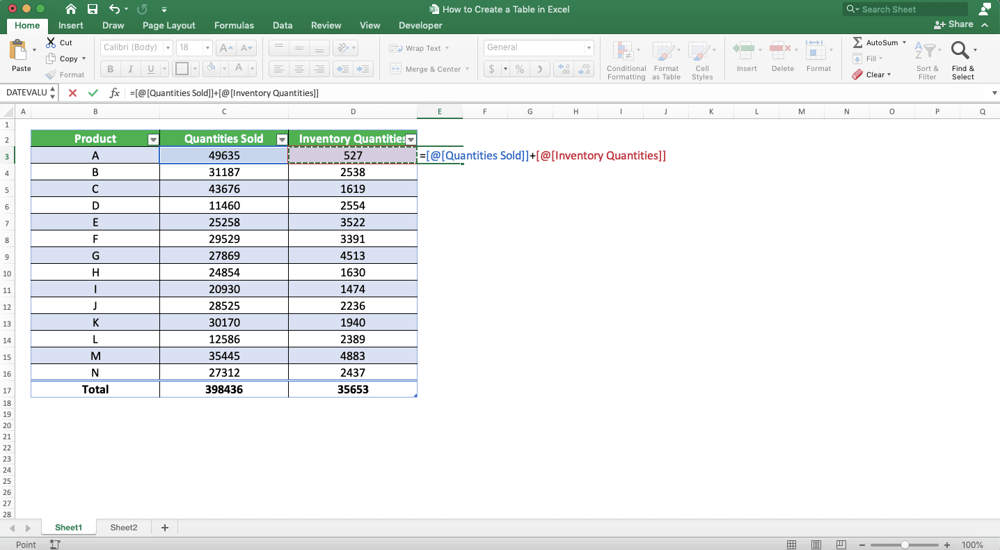
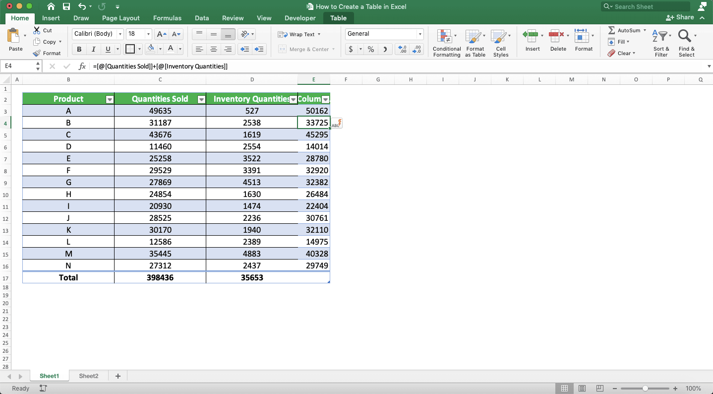
As you enter after you finish writing the formula, Excel will automatically apply the formula to all rows.
How to Name/Rename a Table in Excel
Excel makes it easy to name/rename a table in excel. Just place your cell cursor in your table, and go to the Table tab first. Then, type the name you want for your table in the Table Name text box on the left.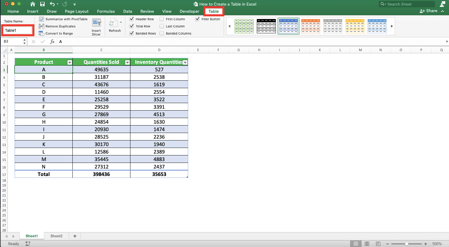
That will name/rename the table for you! You can use the table name when you want to refer to the data in the table later.
How to Refer to Table Columns in an Excel Formula
One occasion when we can refer to our table name is when we write a formula using the table columns. To do that, we can just type the table name and the column header inside square brackets. The process to refer to the data might become simpler for you by doing that!To simplify the understanding, the general writing form when we refer to a table column in a formula is like this.
table_name[table_column_name]
Here is the example when we try to refer to a table column in our COUNTIF writing.
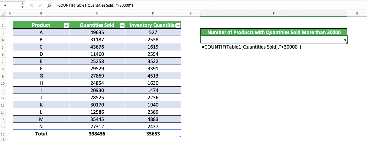
In the example, we want to count the number of products that have more than 30,000 products sold. For this, we need to refer to the data in our table.
As you can see in the formula writing, we refer to the quantities sold column there using Table1[Quantities Sold]. That writing consists of the table name and the column name (from the column header). Using this, we can get our COUNTIF result with no problem!
This should make it easier when we have a large table and we need to refer to some of its columns!
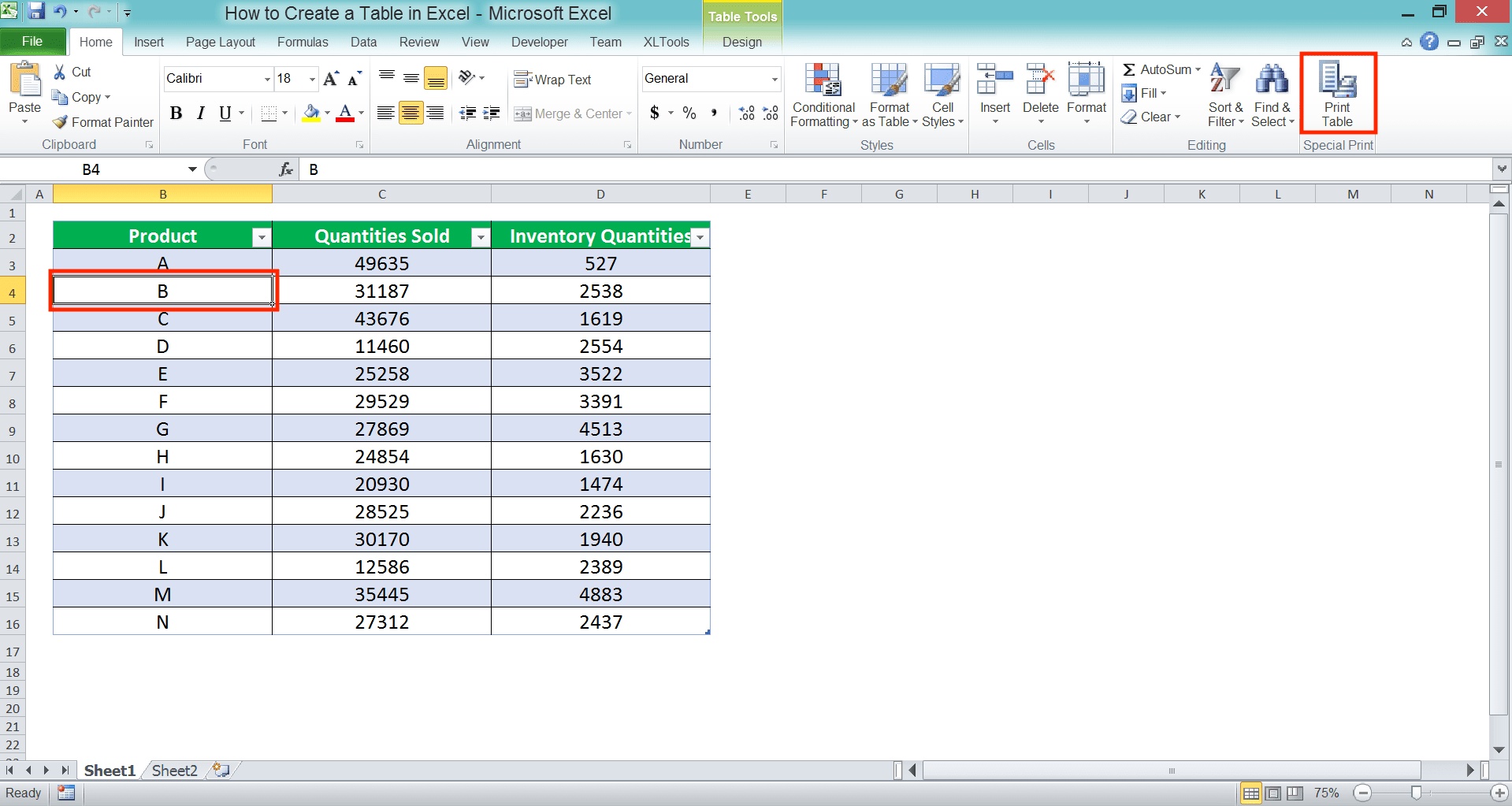
How to Print Only Your Excel Table from Your Worksheet (Only for Windows)
Need to print only your excel table and not the other stuff in your worksheet? You can do that using the Print List command button!However, Excel doesn’t provide the access to this command button by default in its ribbon or quick access toolbar. You need to provide it yourself by customizing your ribbon/quick access toolbar first. You can only add the button in Windows OS, though, as it seems to be not available in Mac.
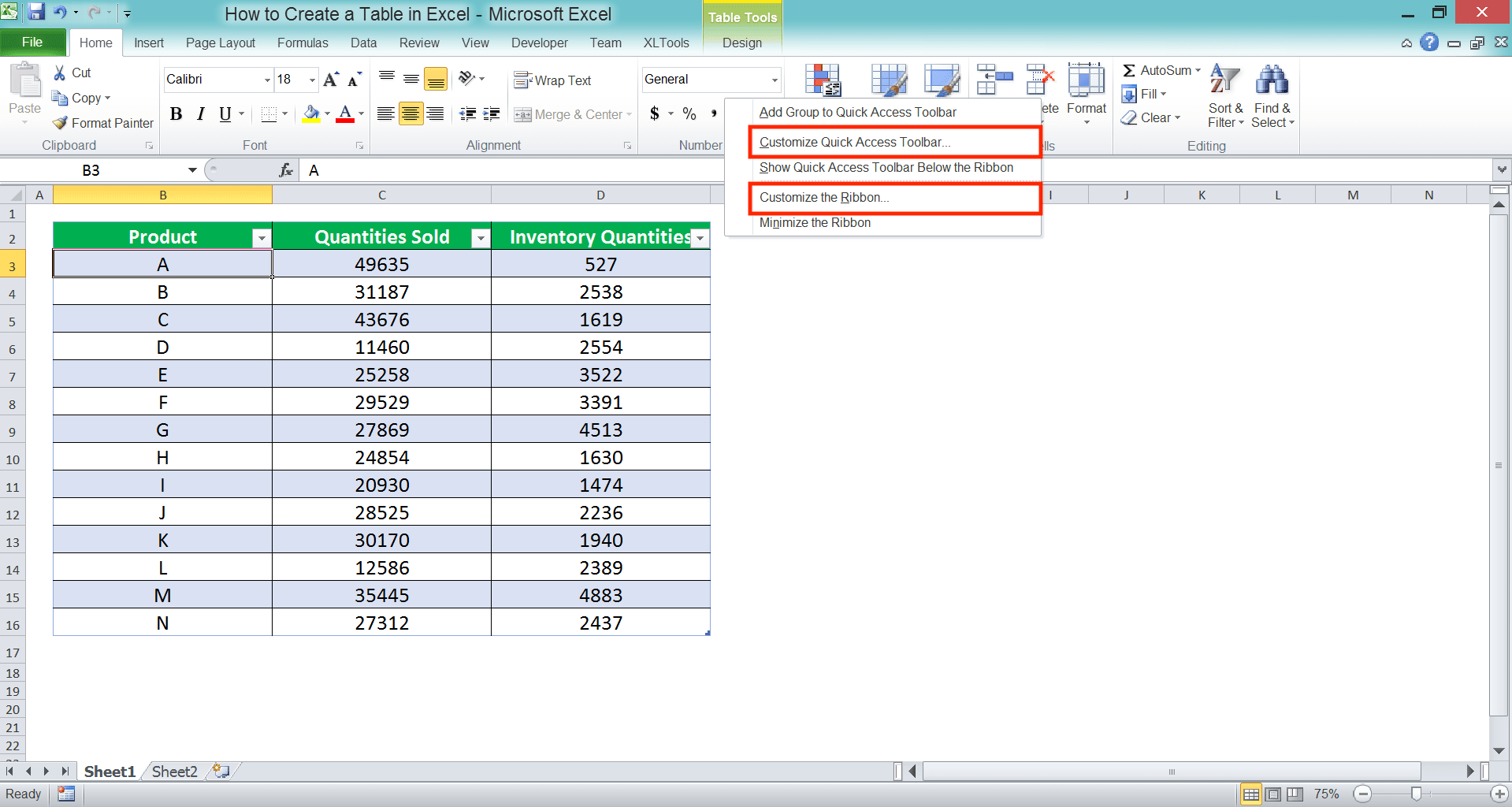
So, how to add the button? First, right-click on your excel ribbon and choose Customize Quick Access Toolbar…/Customize the Ribbon… (depending on where you want to add the Print List button).
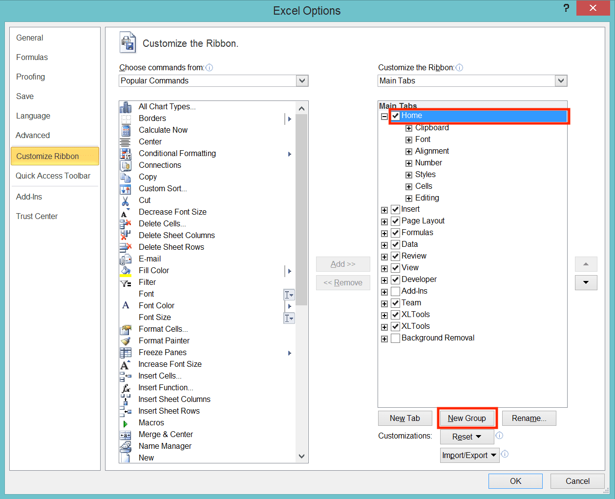
In this example, we want to add the button to our ribbon. In the dialog box that shows up, we need to first add a new group on one of our ribbon tabs. This is because we can only add the button on the ribbon tab group that we create ourselves.
To do that, click on the tab where we want to add the group on the right side of the dialog box. In the example, we add it in the Home tab. Then, click on the New Group button at the bottom.
Excel will create our new group at the most bottom of the tab we choose.
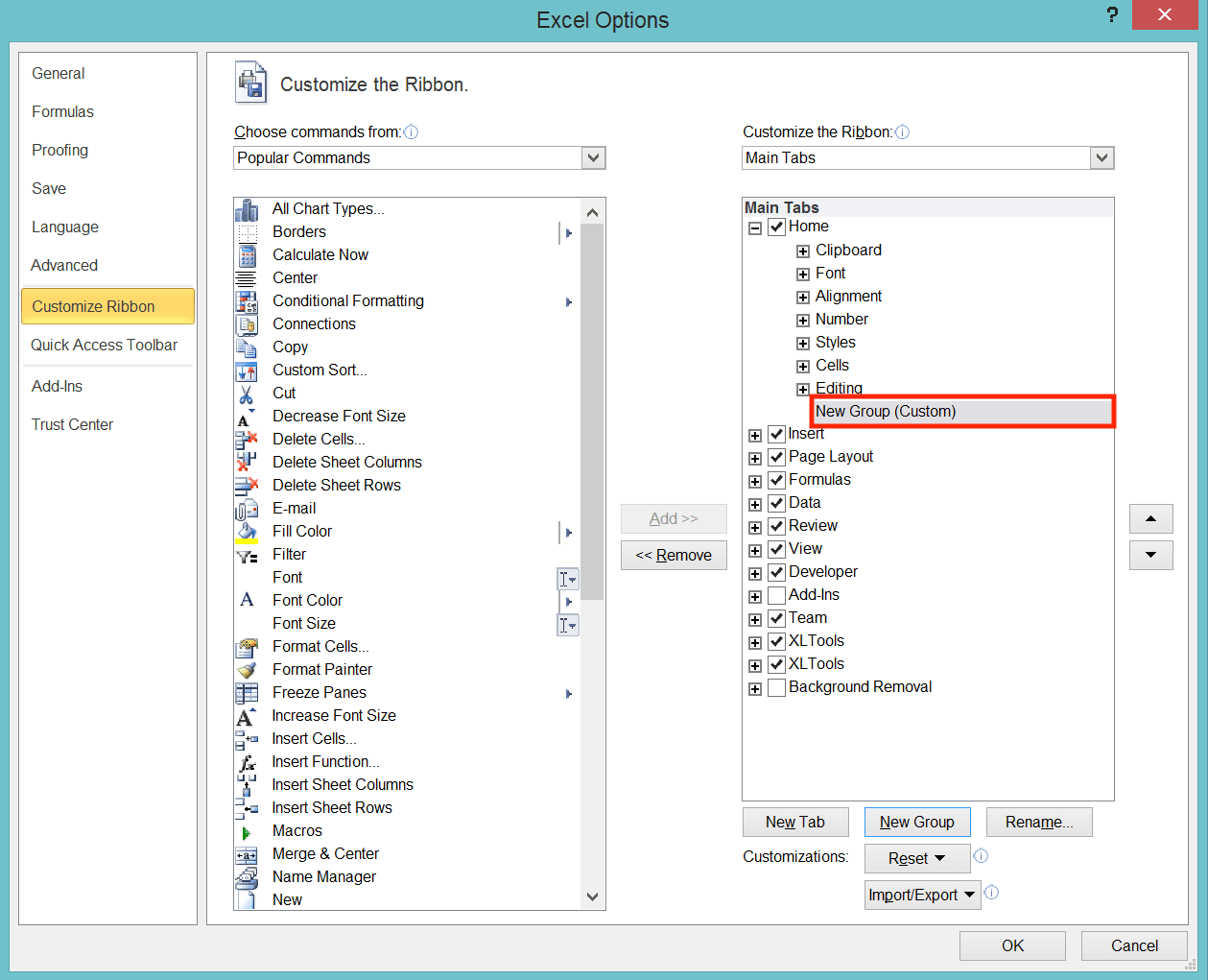
Name the group by right-clicking on it and choose Rename.
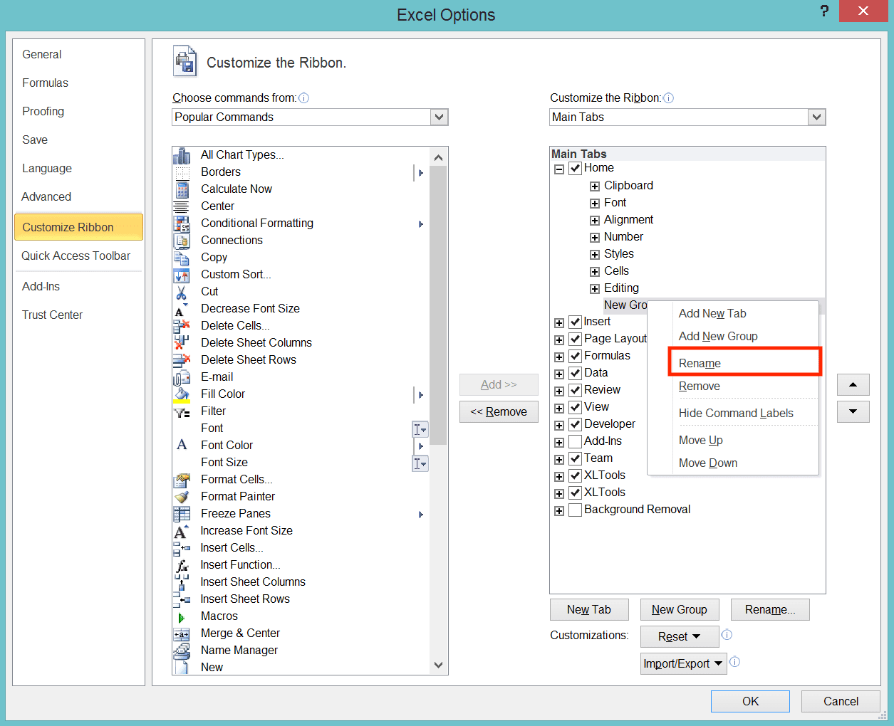
In the example, we name our group as “Special Print”. After that, highlight the group by clicking on it. We will move to set the left side of the dialog box.
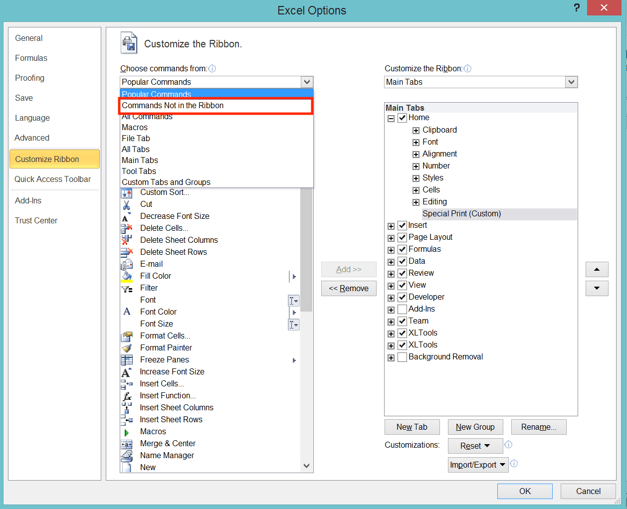
Click the Choose commands from the dropdown on the left. Choose Commands Not in the Ribbon from the dropdown list.
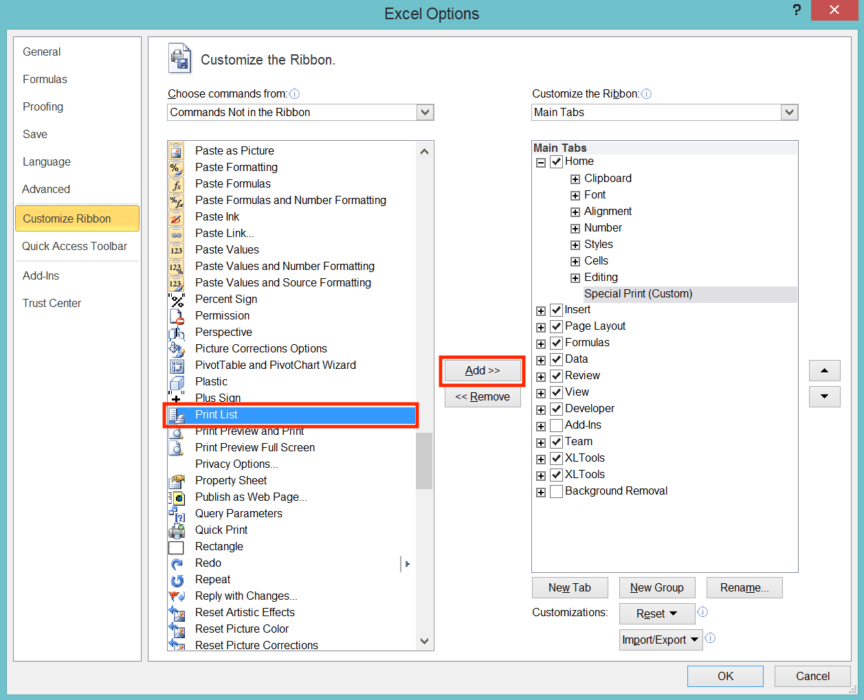
Locate the Print List button in the command button list on the left after you choose that. Then, click on it to highlight it and click the Add >> button in the middle.
Excel will add the button to the group you just make! Click OK and the button will be there in the tab and group you choose.
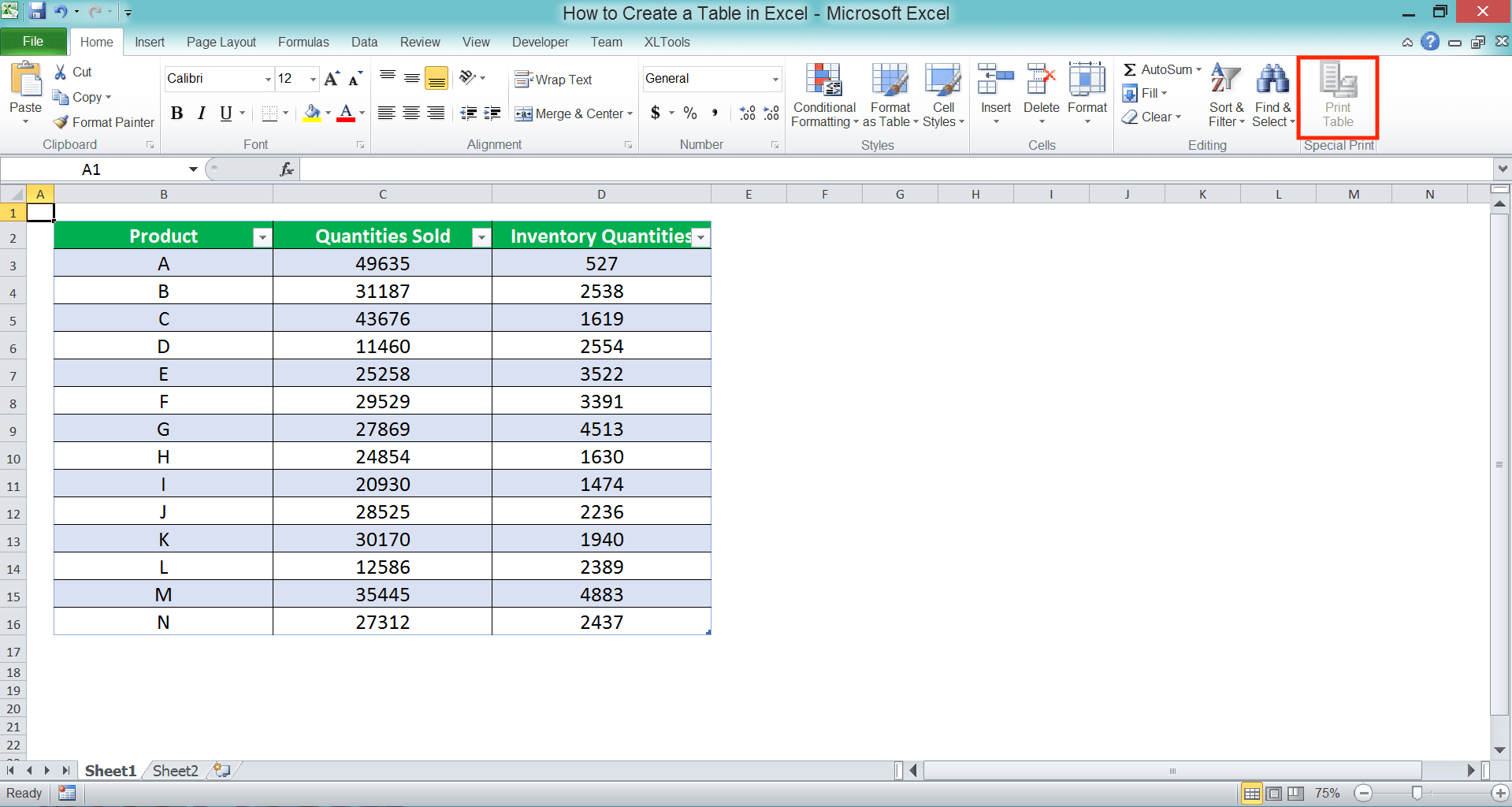
The button will help you to print just the table you want in your worksheet, not anything else. To use the button, place your cell cursor in your table and click the button.
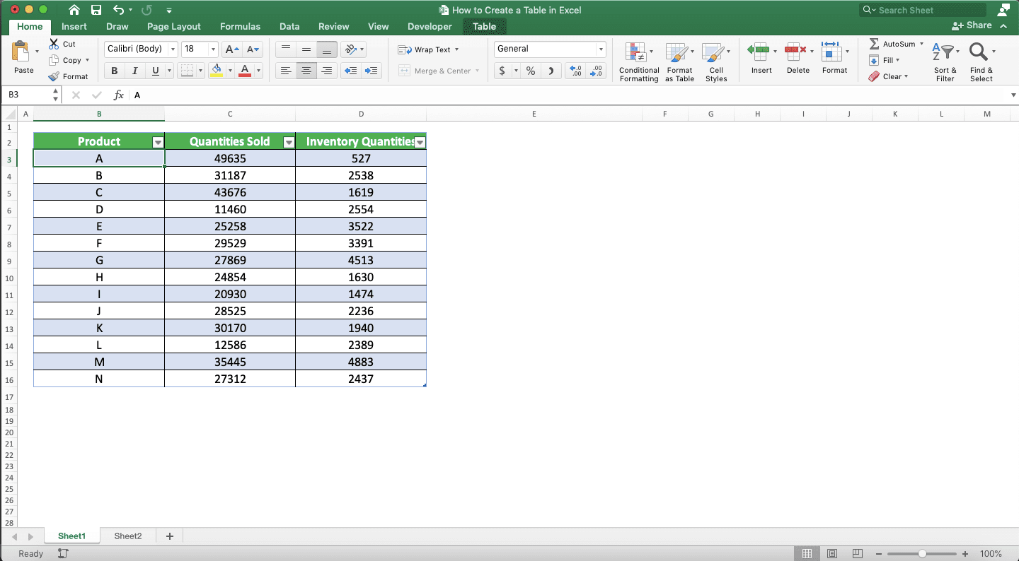
How to Move a Table in Excel
It is quite easy if you want to move a table in excel. Just do it the way you move a normal excel cell range.Put your cell cursor in your table and move your pointer to the table edge. Move it until your pointer changes itself into a hand symbol like this.
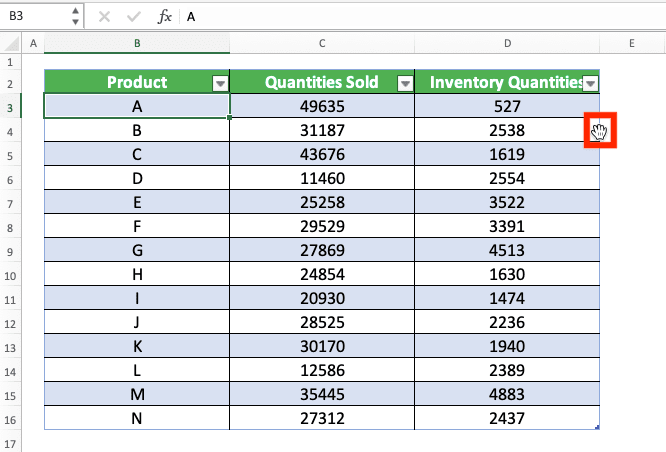
Then, just click and drag your pointer to the place where you want to move your table. You will move your table that way!
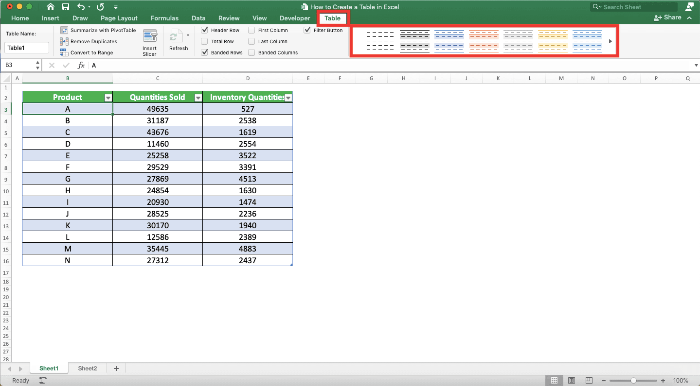
How to Use Table Styles to Change a Table Interface in Excel (How to Color a Table in Excel)
It is also easy to change your excel table interface. Just use the table styles feature that excel has provided for you.Place your cell cursor in the table you want to change the interface on and then go to the Table tab. Next, just choose the table style that suits your preference in the scroll bar on the right.
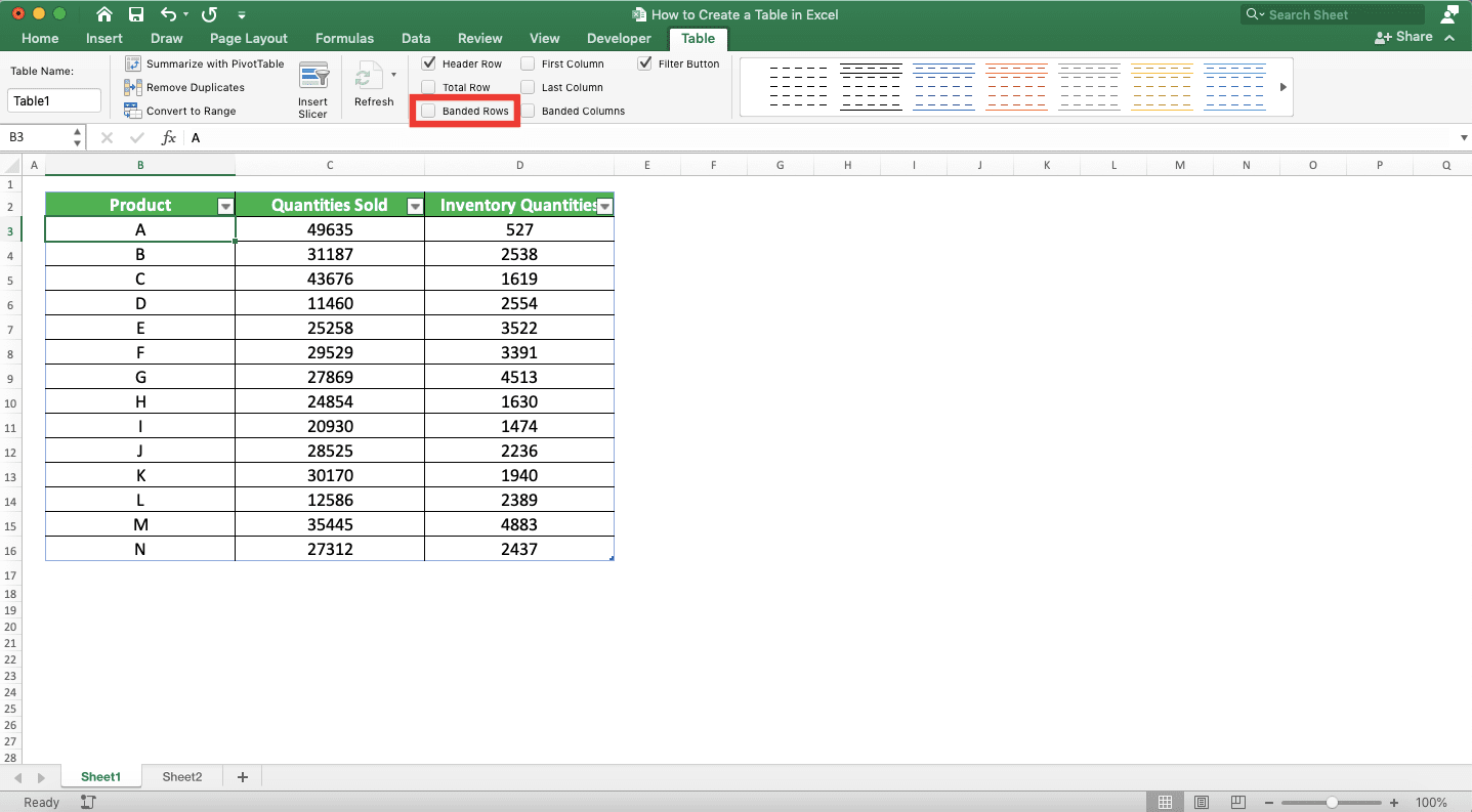
If you want all the rows’ colors to be similar, then just uncheck the Banded Rows checkbox in the tab.
To change your table color beyond what excel provides in its table styles, do it manually. Highlight the table parts you want to custom color and go to the Home tab. Then, click the fill button dropdown and choose the color you want.
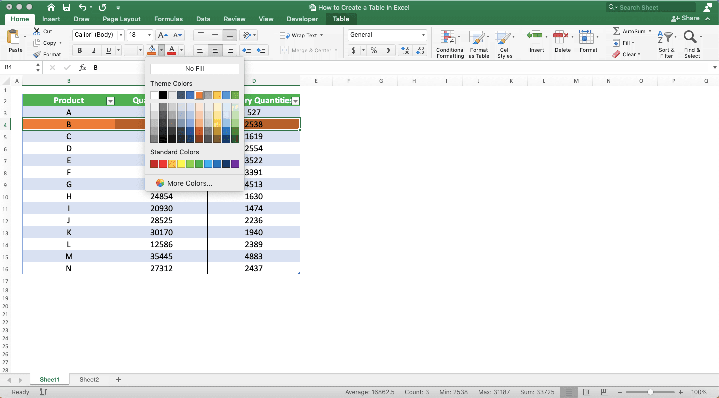
Just like when you color cells in your worksheet!
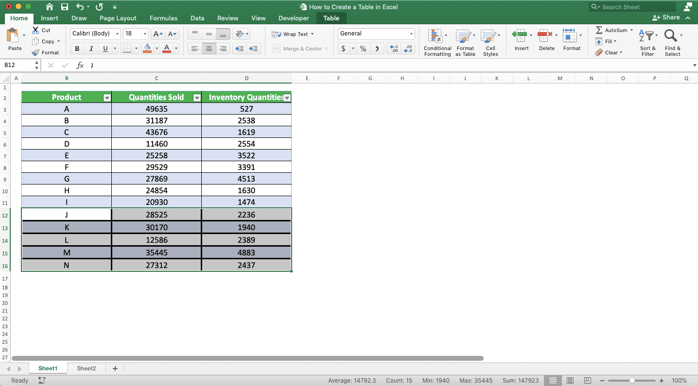
How to Make and Thicken a Table Border Line in Excel
If you want to custom the border lines in your table, then custom them like the usual cell border lines too.Highlight the cell range in the table where you want to custom the border lines. Then, go to the Home tab and click the border button dropdown. You can choose the available border lines settings there, draw them yourself, or custom them by clicking More Borders…

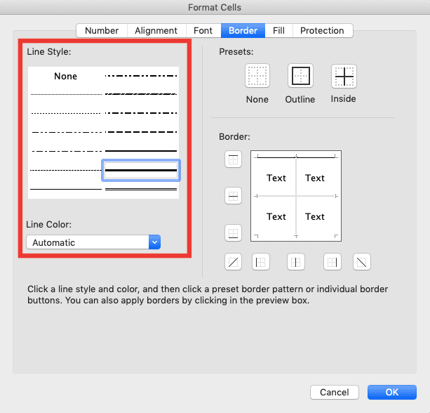
If you decide to click More Borders…, then you can custom the border lines in your table more freely. On the left side of the dialog box that shows up, you can select the line style/thickness and color.
When you have determined the line you want, add it on the right side. Click on the presets or in the border menu below. You can also remove the border lines you want by doing that.
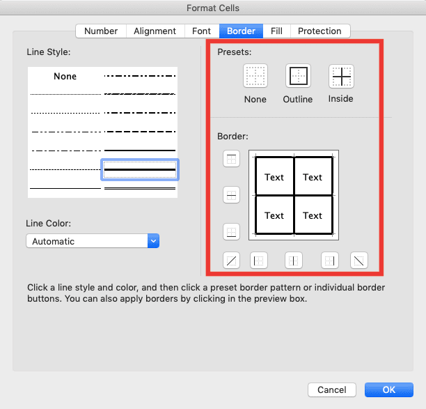
After you are done, click OK. The border lines on the table part you highlight have changed themselves to the way you set them!
How to Increase/Reduce a Table Size in Excel
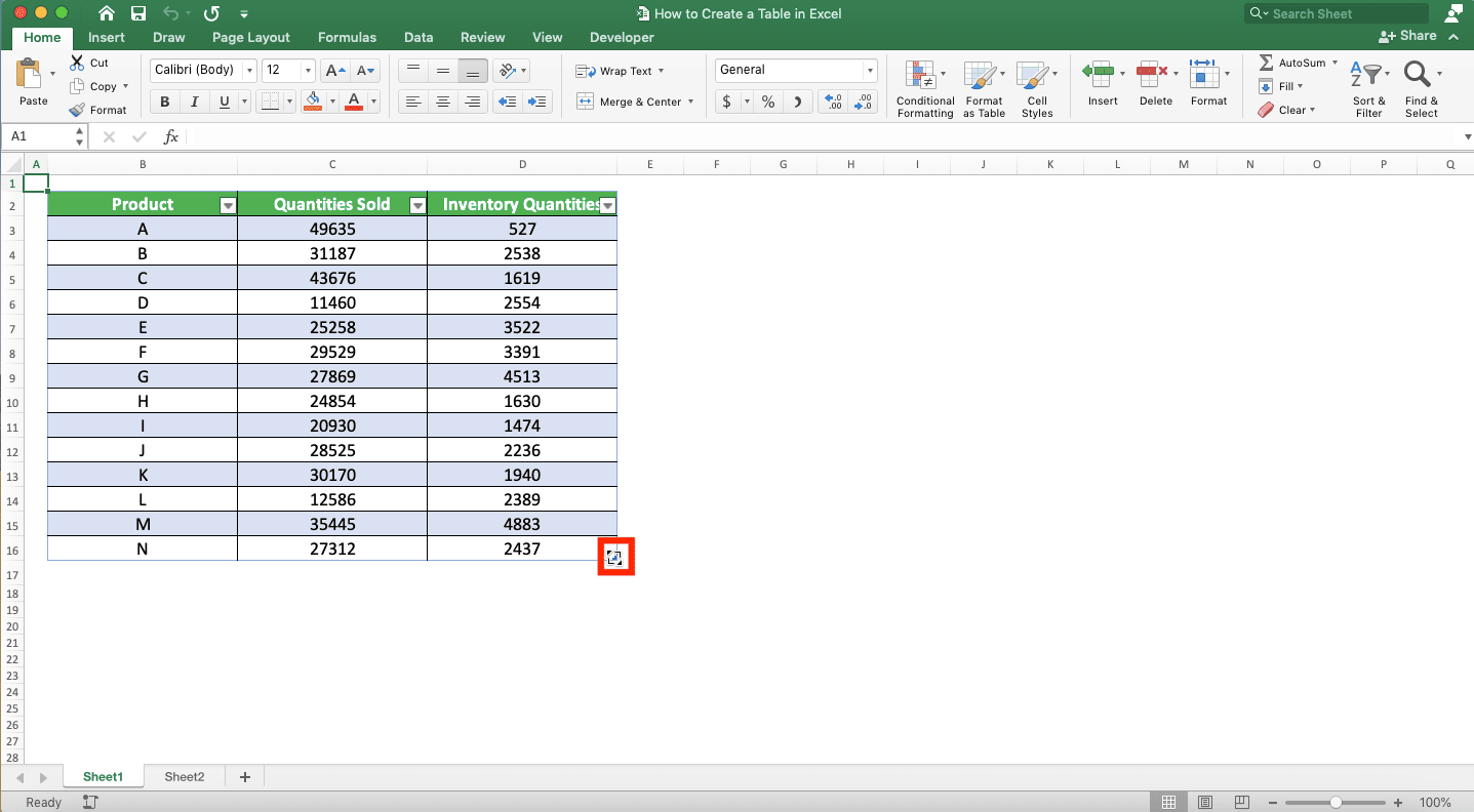
To increase/reduce a table size in excel, notice a little mark at the bottom right of your table.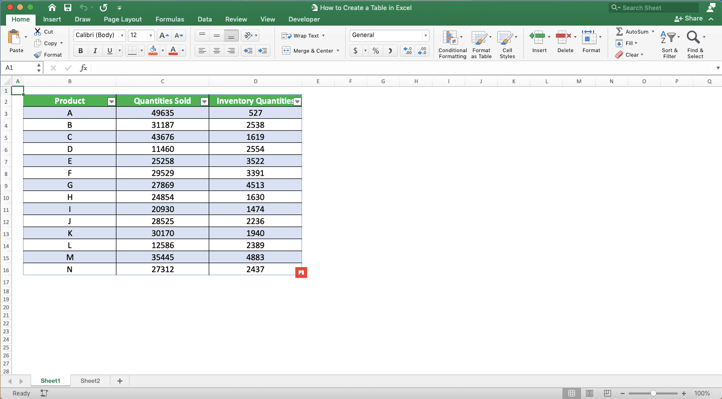
Move your pointer to its location until it changes form.
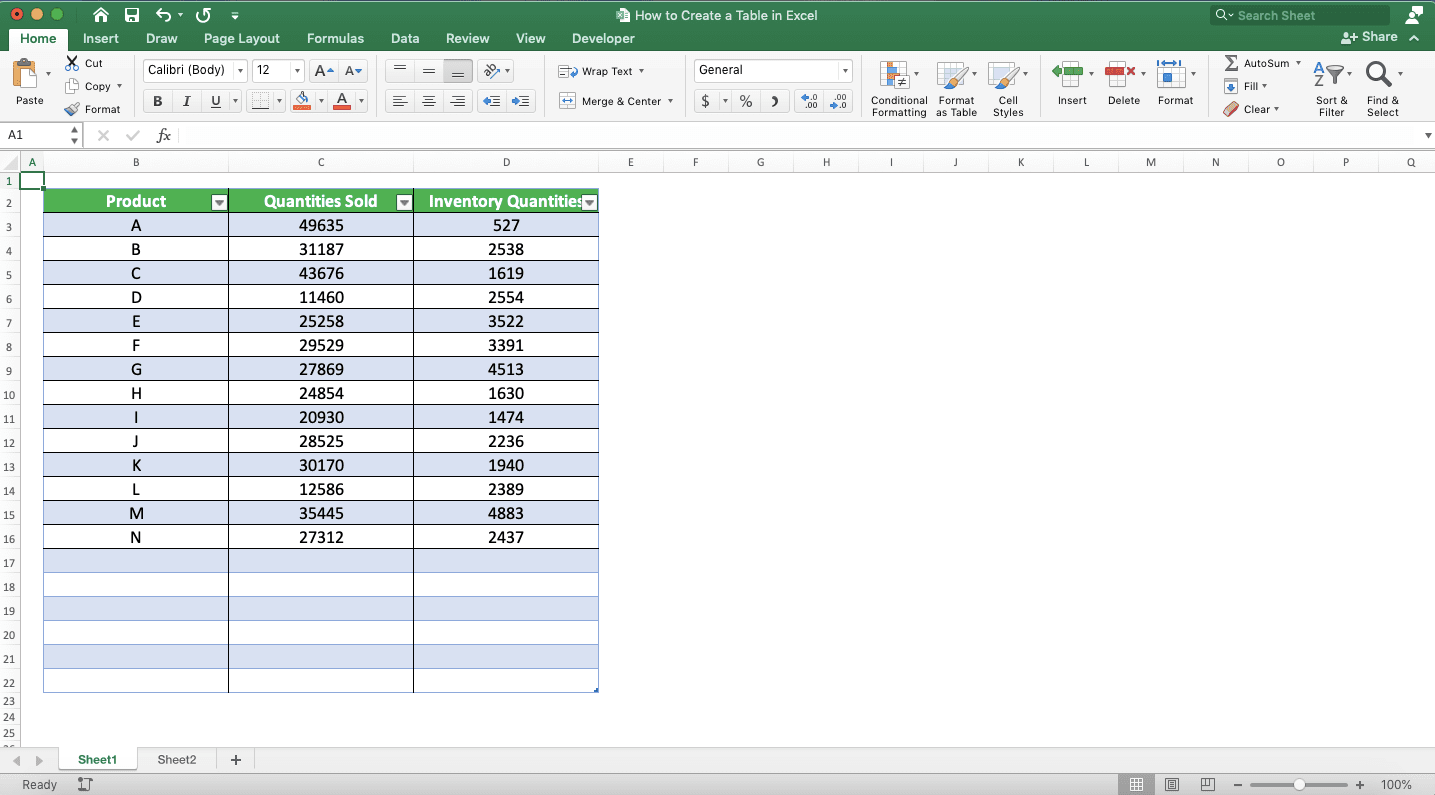
Click and drag until you get the table size you want. Release your drag and you have resized your table!
How to Join/Combine Tables in Excel
Do you have more than one table and you need to combine their data into one table? If you want to combine the rows and those tables have similar headers, then you just need to copy and paste.However, if you want to combine the columns, then you need to have one same column in both tables. This column will act as a bridge for the tables combination process. The data in each row of the column should also be unique.
If you have that kind of column, then you can combine your tables using INDEX MATCH. We use INDEX MATCH just in case the data between both tables same column isn’t in the same order. The writing form of INDEX MATCH for the purpose is as follows.
= INDEX ( column_to_combine , MATCH ( reference_value_in_table_1 , same_column_in_table_2 , 0 ) , 1 )
Put the INDEX MATCH formula in the table which becomes the place where you combine your tables’ data. Put it in one column and in each row of that column.
For the INDEX cell range input, we input the column of the second table (the table which data we pull to the first table to combine the tables data) that we want to combine.
In the MATCH formula inside INDEX, we input the reference value to pull the data from the second table. The reference value is the cell value which is parallel with the cell where we put our INDEX MATCH. The value must come from the same column between the first table and the second table.
We also input the same column cell range from the second table and 0 for exact search mode in the MATCH. By doing that, we can pull the right data from the column we want to combine to the first table. Then, we input 1 in our INDEX because we only have one column we give as the INDEX cell range input.
If you write the INDEX MATCH using that pattern, you will be able to combine your tables easily! As the excel table copies the formula we write across all rows, we just need to write our INDEX MATCH once.
To illustrate the INDEX MATCH concept in this tutorial part, let’s say we have these two tables we want to combine. We put them in separate sheets in our excel workbook.
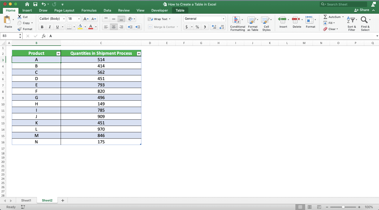
We want to combine the quantities in shipment process column in the second table to the first table. As both tables have the product column, we can use INDEX MATCH to combine them.
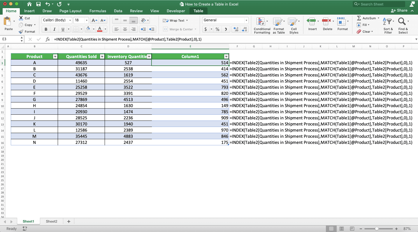
Write INDEX MATCH on the right of the table where you want to get your combination result. Use the writing form we have discussed earlier.
Remember that the excel table will copy the formula we write next to it across all of its rows. When we finish writing one INDEX MATCH formula for the combination process in the example and enter, we immediately get this.
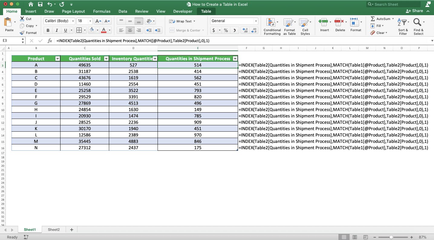
We have combined the data that we want from the two tables! Next, just format the combination column a bit so it becomes like a genuine part of our table!
How to Lock a Table in Excel
To lock a table in excel, you need to do what you do when you lock cells in excel. That is we need to make sure we enable the table cell range lock mode and we must protect our sheet.Have you mastered the way to do that? Here are the steps if you haven’t.
First, highlight your table cell range. Right-click on it and choose Format Cells….
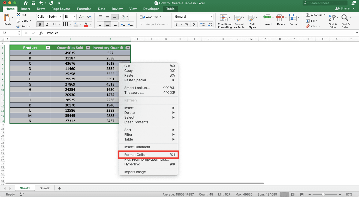
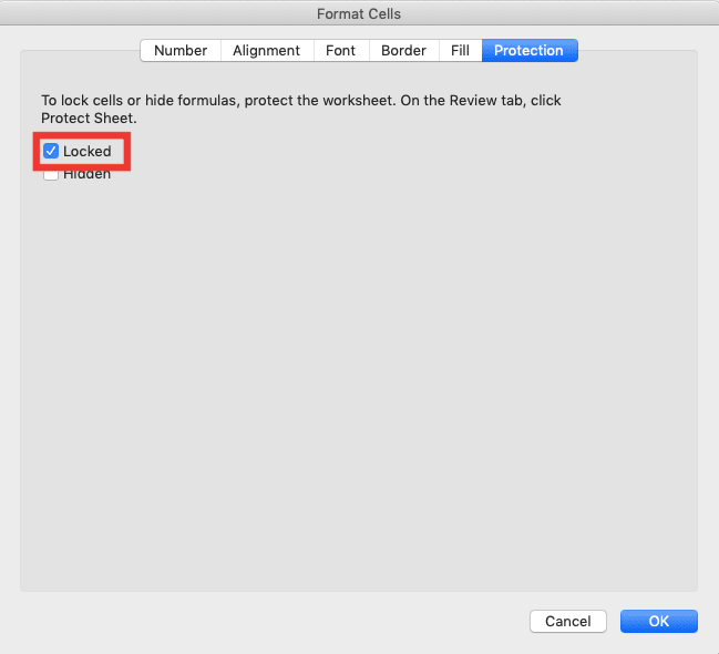
In the dialog box that shows up, go to the Protection tab. In the tab, make sure the Locked checkbox there is checked. After that, click OK.
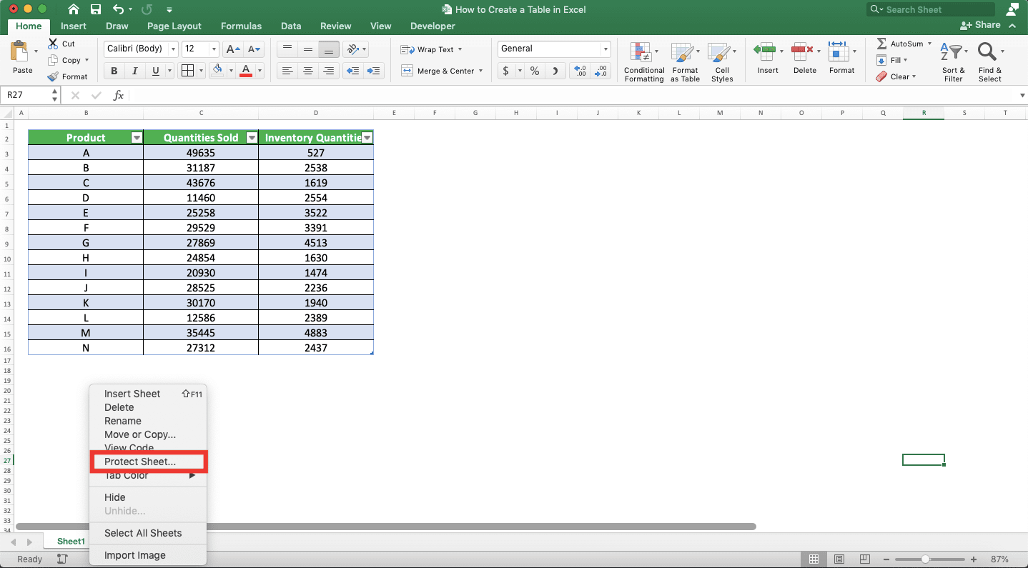
Now, we just need to protect the worksheet where the table resides. To do that, right-click on the sheet tab at the bottom left and choose Protect Sheet….
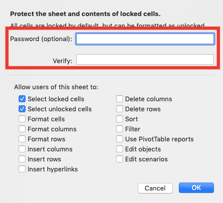
Enter a password if you want, twice in the text boxes of the dialog box that shows up. Excel will ask for the password when you want to unprotect the sheet later. Don’t enter anything in the text boxes if you don’t want to enter a password for that.
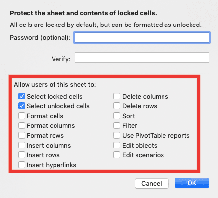
Set what things you allow and not allow in the protected worksheet in the bottom part of the dialog box too.
After all are set, click OK. By doing those steps, you have locked your table!
If you want to unlock the table, then just unprotect the sheet again. And if you want to protect just the table, then you need to disable the lock mode in other cells (to highlight all the cells quickly to set their lock mode, you can press Ctrl + A in your keyboard).
How to Remove a Table Formatting in Excel
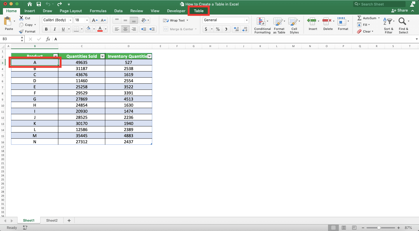
Want to remove your table formatting but want to keep applying the table feature? Say no more, we have got you covered.To do that, place your cell cursor anywhere in your table first. Next, go to the Table tab in your ribbon.
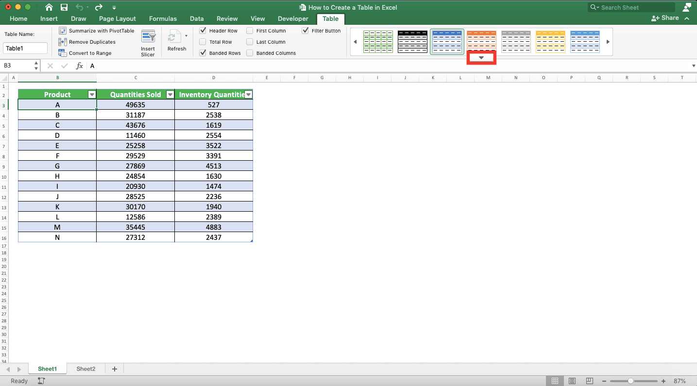
In the table styles scroll bar, click the down arrow button.
In the dialog box that shows up, click Clear.
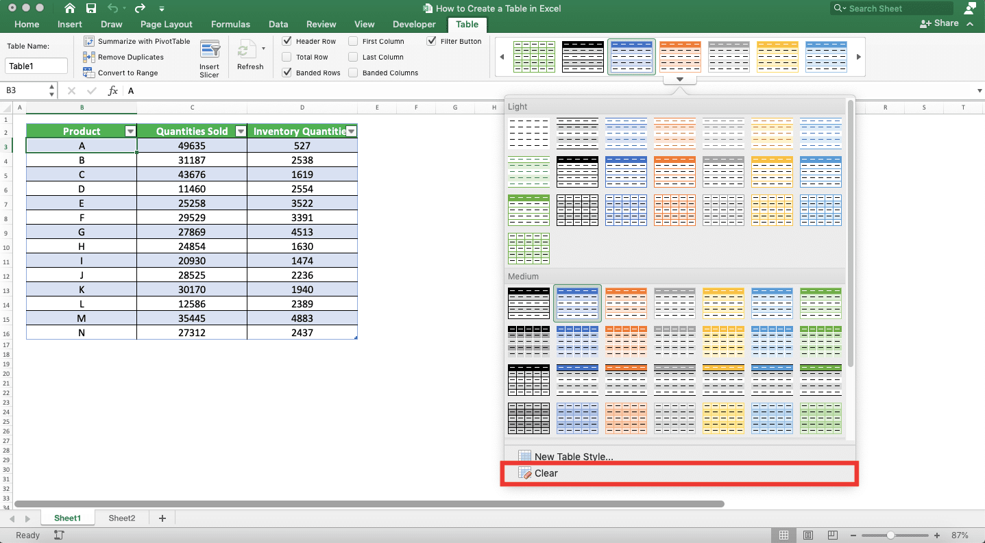
By doing that, you have removed the formatting of your table but your table will still be there!
How to Remove a Table in Excel
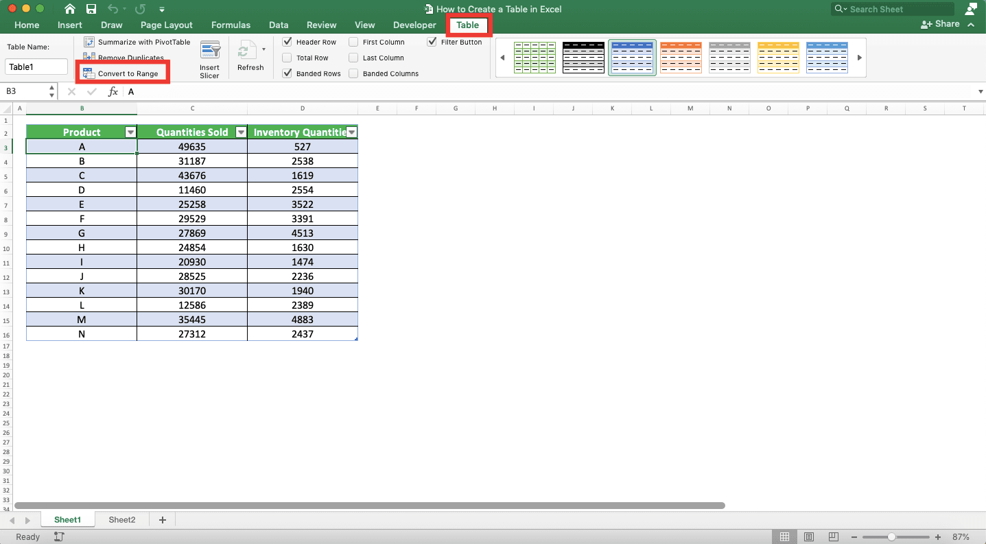
Do you want to just convert your table back into a normal cell range or delete the contents too? We will discuss the method to do both of them separately in the following.First, let’s discuss how to convert a table into a normal cell range. Place your cell cursor anywhere in your table and go to the Table tab. In the Table tab, click the Convert to Range button.
Choose Yes in the dialog box that shows up.

You will immediately convert your table back into a normal cell range!
Easy, right? What if you want to delete the contents too? The method to do that is quite easy as well.
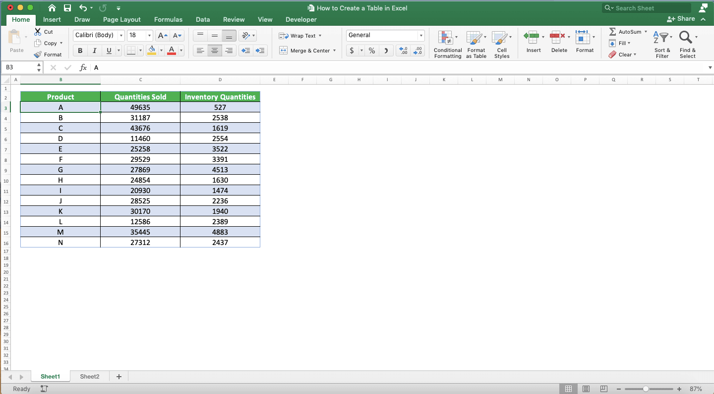
First, highlight your table cell range. Then, go to the Home tab and click the Clear button dropdown there. Choose Clear All from the dropdown list.
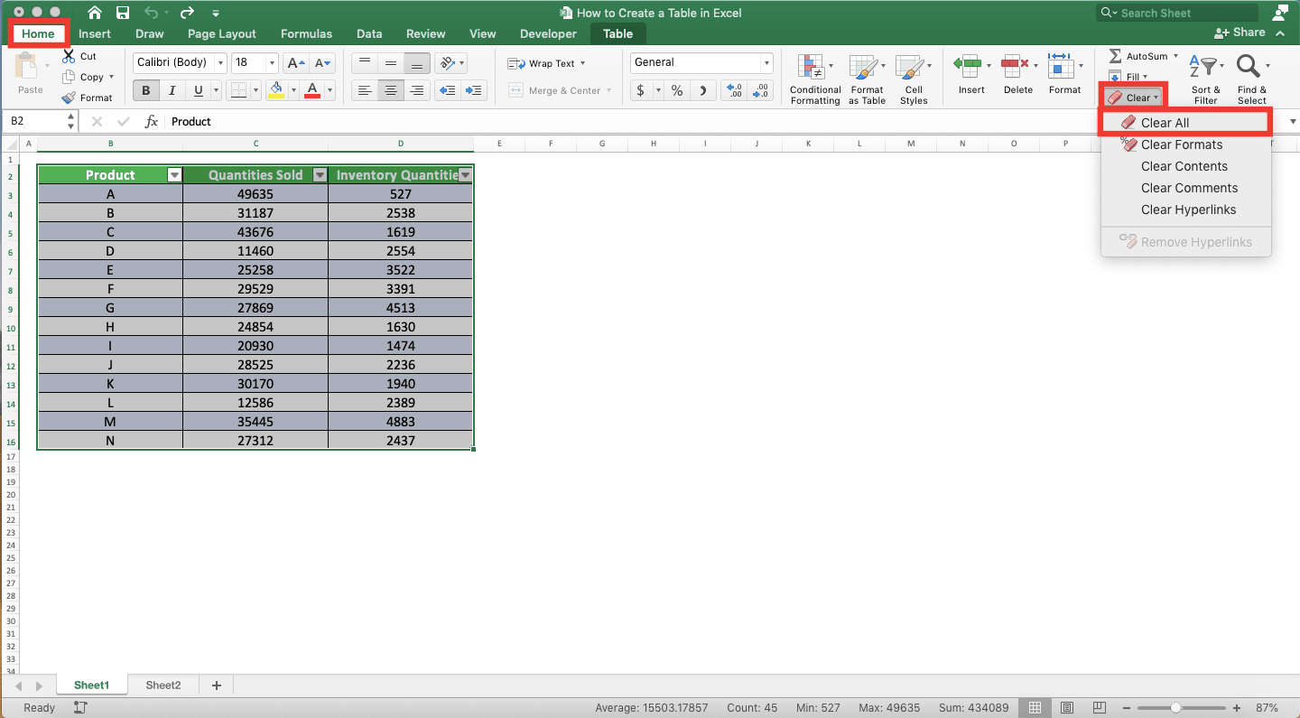
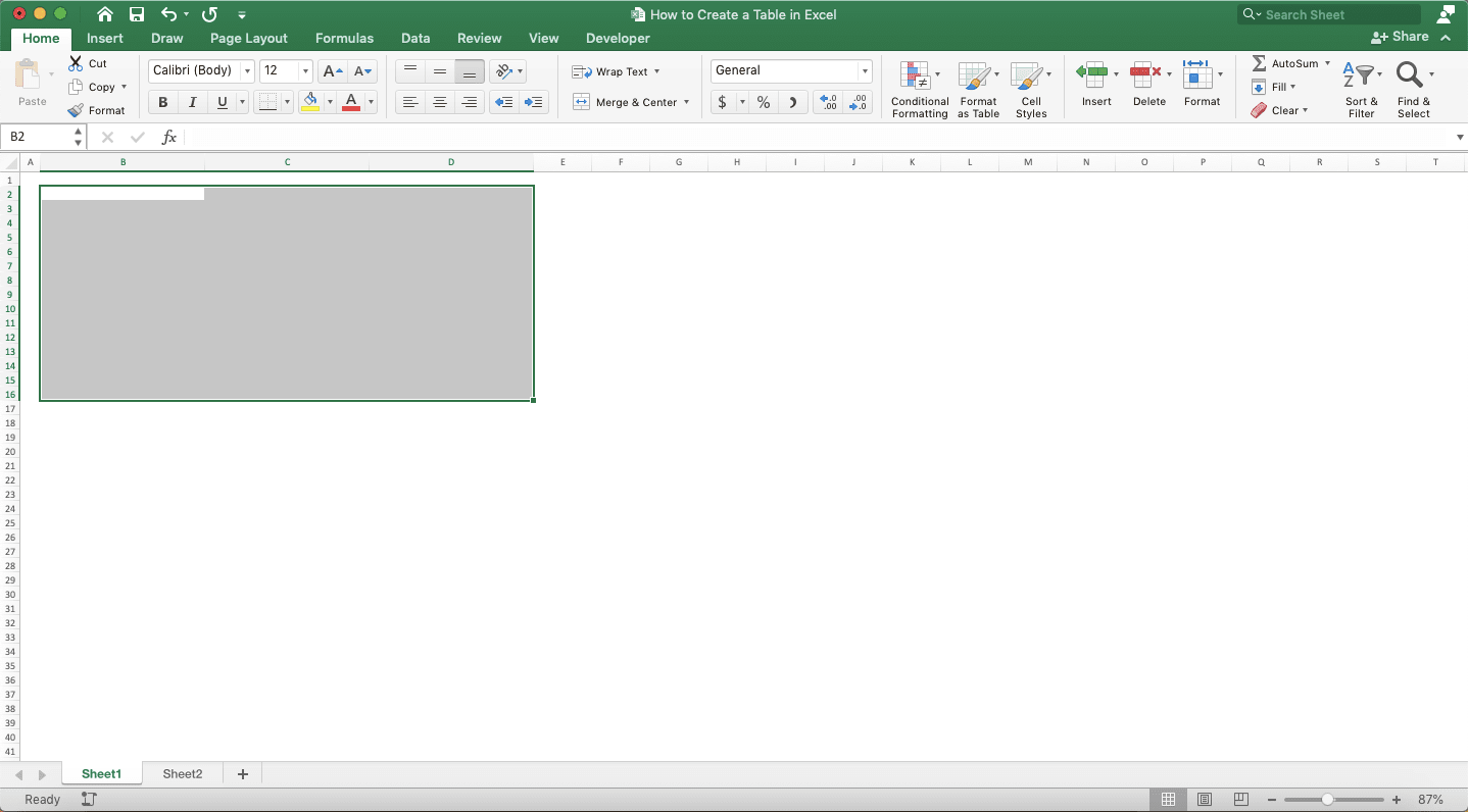
By doing that, you have deleted your table with its content too!
Exercise
After you learned completely how to make a table in excel the way you want, let’s do an exercise. This is so you can sharpen your understanding of the excel table feature in excel.Download the exercise file and do the instructions. Download the answer key file if you have done the exercise and want to check your answers. Or probably when you are confused about what to do with the exercise instructions!
Link to the exercise file:
Download here
Questions
- Convert the cell range in sheet1 and sheet2 into tables! Style the tables the way you prefer!
- Combine the two tables’ data in sheet1!
- Average the score test 1 and 2 and get the standard deviation of the score test 3! Use the excel table’s total row feature to get them!
You can use the table in this exercise to practice other excel table features you want!
Link to the answer key file:
Download here
Additional Note
If you often use a cell range with columns as your formulas references, then you should apply the excel table feature. Doing that will make it easy for you to input the cell range and refer to new data later.Related tutorials you should learn: