How to Use INDEX MATCH in Excel: Functions, Examples, and Writing Steps

In this tutorial, you will learn all about INDEX MATCH in Excel.

When we work in Excel, we may often need to find certain data from the data tables that we have. To do that, many of us may opt to use the VLOOKUP function.

However, VLOOKUP has some limitations that might make us unable to find the data we want. To solve that problem with VLOOKUP, one of the best solutions provided by Excel is to combine INDEX and MATCH functions into a formula. By combining them, we can find our data with much more flexibility. We might even prefer to use INDEX MATCH rather than VLOOKUP when we need to find data again in Excel in the future.

What is this INDEX and MATCH combination and how to use it properly in Excel? If you want to learn, read this article until its last part.

Disclaimer: This post may contain affiliate links from which we earn commission from qualifying purchases/actions at no additional cost for you. Learn more

Want to work faster and easier in Excel? Install and use Excel add-ins! Read this article to know the best Excel add-ins to use according to us!

The Use of INDEX MATCH in Excel

We can use the INDEX and MATCH combination in Excel to find and get data from a cell range (usually in the form of a data table) vertically and/or horizontally.

The INDEX MATCH Result

The result we get from INDEX MATCH is the data we want to find

The Excel Version from Which the Combination of INDEX and MATCH Can Be Used

We can use both INDEX and MATCH functions since Excel 2003. Thus, that is the earliest Excel version from which we can use INDEX MATCH.

How to Write INDEX MATCH and Its Inputs

Here is the general writing form of INDEX MATCH in Excel.



The formula above assumes that you want to find your data vertically (the same data-finding behavior as VLOOKUP). If you want to find data horizontally, put the MATCH formula in the place of the third INDEX input and change the MATCH formula in the second INDEX input into a number that indicates the index number of the row from where you want to get the INDEX MATCH result from the cell range you input in the first input of INDEX. If you want to find data vertically and horizontally, you should put the MATCH formula in the second and third inputs of the INDEX function.

Here is a brief explanation of the inputs given in our general writing form of INDEX MATCH above.

• cell_range_reference = the cell range reference where you want INDEX MATCH to find your data
• value_reference = the value that becomes the reference for MATCH to find the row position of the data you want to find with INDEX MATCH in your referred cell range
• column_reference = the column where the reference value you input earlier in MATCH is in
• [match_type] = optional. The behavior of MATCH when it tries to find the position of your reference value. Input 0 to find an exact match, -1 to find an exact match or a larger value closest to the reference value, or 1 to find an exact match or a smaller value closest to the reference value. The default input here is 1
• result_column_number_in_cell_range = the index number of the column in the referred cell range in which you want to find your INDEX MATCH result

Here are several points you may want to pay attention to about the INDEX MATCH inputs.

• Ensure that the referred cell range you input in INDEX and the referred column/row you input in your MATCH are proportional so you won’t get the wrong result from your INDEX MATCH


• For the match_type input of MATCH, you may want to make sure you input 0 all the time if you don’t want to find a value other than the exact match of your MATCH’s reference value. This should ensure MATCH won’t find the wrong row/column position of the data you want to find with your INDEX MATCH


• If you use -1 for the match_type input of MATCH, the column/row reference that you input in it must be sorted in descending order so you can get the correct MATCH result. On the other hand, if you use 1, the column/row reference must be sorted in ascending order


• If you want to find your data only vertically/horizontally (not vertically and horizontally), you may want to input only one column/row as your INDEX first input to make your INDEX MATCH formula much simpler

The Example of Usage and Result

Here is an implementation example of INDEX MATCH in Excel.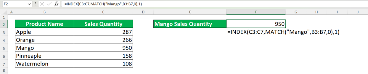



In this example, we use INDEX MATCH to get mango sales quantity. In the INDEX MATCH, our MATCH formula is used to determine the row position of the mango sales quantity we want to get from our data table.

We input the cell range of the “Sales Quantity” column in the data table as our first input for INDEX. This is because the data we want to get from our INDEX MATCH is sales quantity data. Then, as we use MATCH to get the row position, we type our MATCH formula in the second input position of INDEX.

In the MATCH formula, we type “Mango” as our reference value as we want to get mango sales quantity from our INDEX MATCH. Next, we input the cell range of the column where the “Mango” word is in the data table as we want to get the row position of the “Mango” word in that column. Last but not least, we input the number 0 as we want to get an exact match for the row position.

In the last INDEX input, we input 1 as we only input one column as the cell range reference of our INDEX formula. After we have typed all of that, we get the mango sales quantity we want from our INDEX MATCH formula!

What about if we want to find the mango sales quantity horizontally? Here is an example of the INDEX MATCH implementation for that case.



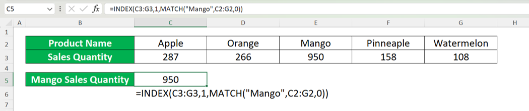
As we have discussed in the previous section of this article, we just need to write our MATCH formula in the third input of our INDEX in this case. We also change the first input of our INDEX to the cell range of the row where the sales quantity data is and the second input of our INDEX to 1 (as we only input the cell range of one row in our INDEX first input). The result of the formula writing is the mango sales quantity too.

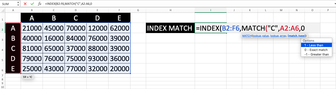
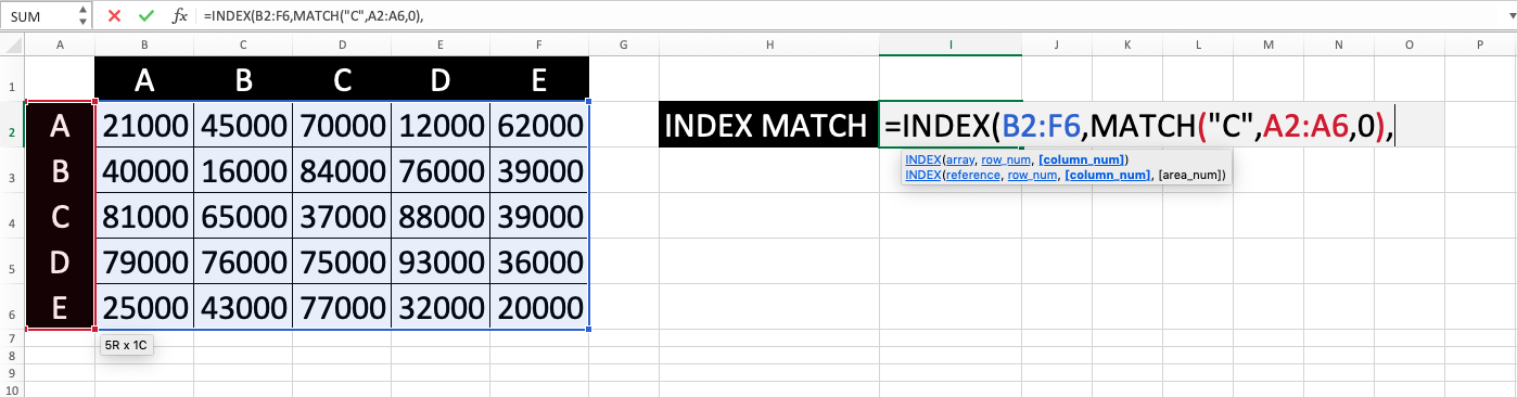
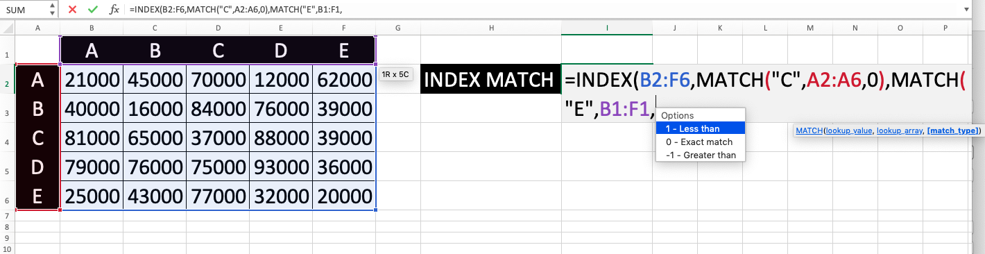
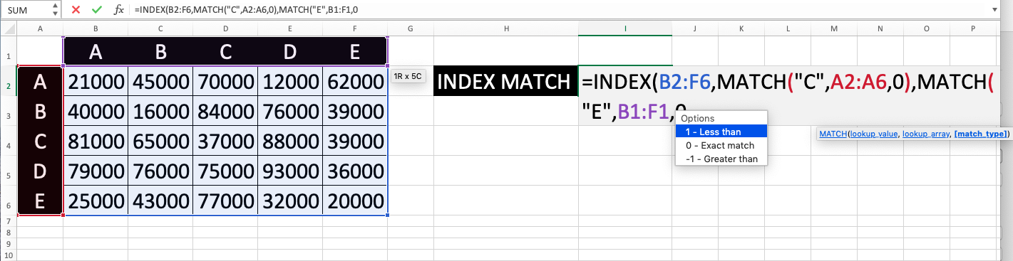
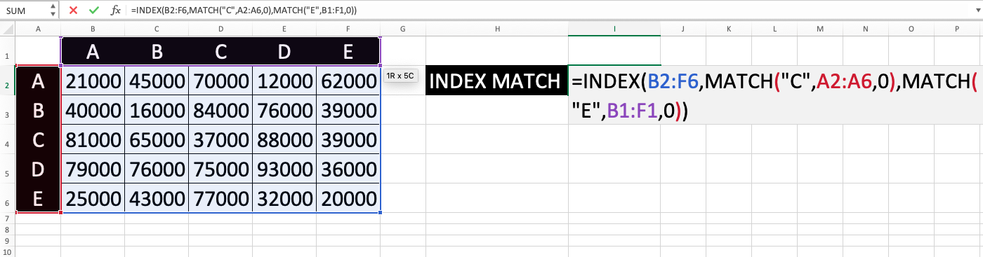
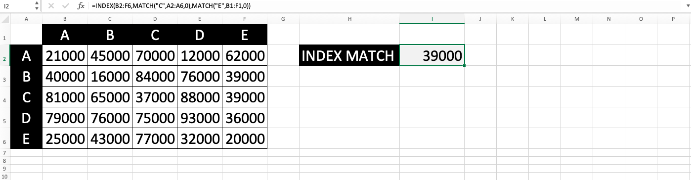
Here is an implementation example of INDEX MATCH if we look for our mango sales quantity data vertically and horizontally.



As you can see in the example, in this case, we write MATCH formulas as the second and third inputs of our INDEX formula. For the first input of our INDEX, we input the cell range of our data table as we want to look for our data not only in one row or one column. The result is similar to our two previous cases, the mango sales quantity data.

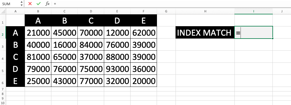
Writing Steps

After we have learned the implementation examples of INDEX MATCH in Excel, let’s learn about the writing steps of its formula in detail. For this part of the article, we assume that we want to find our data vertically and horizontally.

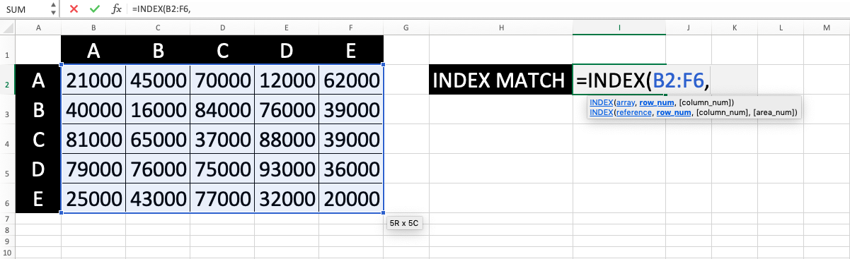
1. Type an equal sign ( = ) in the cell where you want to put your INDEX MATCH result in
   
   
   
   
2. Type INDEX (can be with small and/or large letters) and an open bracket sign
   
   
   
   
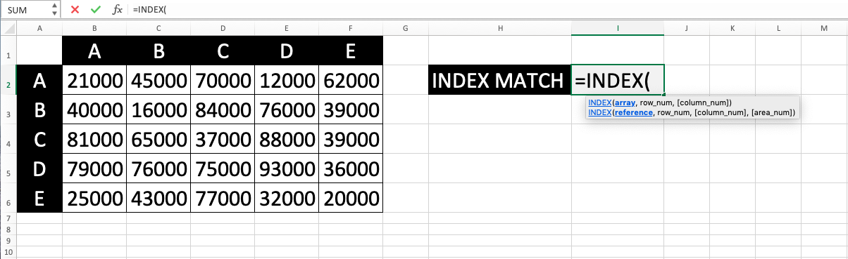
3. Input the cell range where you want to find your data. Then, type a comma sign ( , )
   
   
   
   
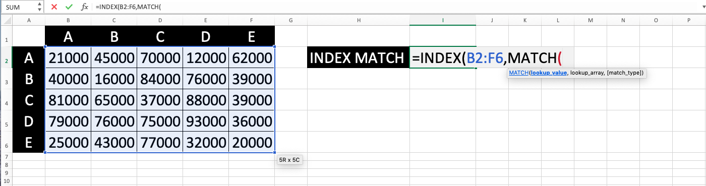
4. Type MATCH (can be with small and/or large letters) and an open bracket sign
   
   
   
   
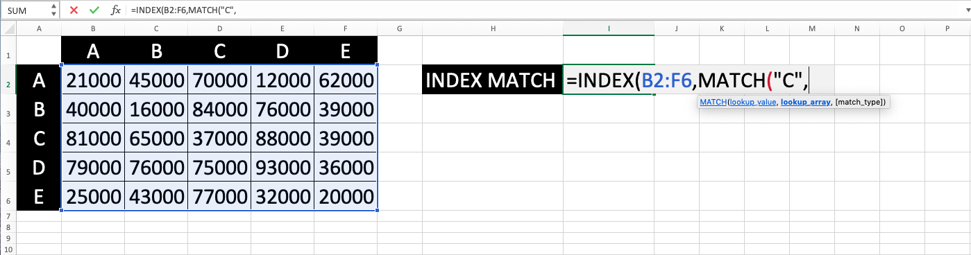
5. Input the value that you want to find to determine the row position of the INDEX MATCH result in your referred cell range. Then, type a comma sign
   
   
   
   
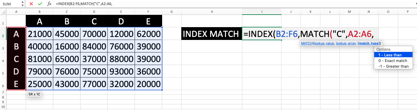
6. Input the cell range of the column where you want to find the reference value of your MATCH. Then, type a comma sign
   
   
   
   
7. Optional: Input the match type you want MATCH to adhere to when trying to find its reference value (0 for an exact match, -1 for an exact match or a larger value closest to the nearest value, and 1 for an exact match or a smaller value closest to the nearest value)
   
   
   
   
8. Type a close bracket sign and a comma sign
   
   
   
   
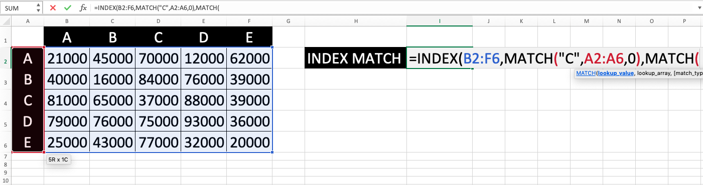
9. Type MATCH (can be with small and/or large letters) and an open bracket sign
   
   
   
   
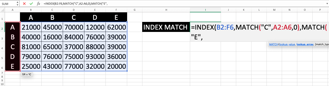
10. Input the value that you want to find to determine the column position of the INDEX MATCH result in your referred cell range. Then, type a comma sign
    
    
    
    
11. Input the cell range of the row where you want to find the reference value of your MATCH. Then, type a comma sign
    
    
    
    
12. Optional: Input the match type you want MATCH to adhere to when trying to find its reference value
    
    
    
    
13. Type a close bracket sign twice
    
    
    
    
14. Press Enter
15. Done!
    
    
    
    

INDEX MATCH vs VLOOKUP

If we use INDEX MATCH, then we probably don’t need to use VLOOKUP anymore as they can do the same thing in Excel, which is finding data for us from a cell range. But, should we use INDEX MATCH instead of VLOOKUP? What are the differences between the two?



If you ask us, then our recommendation is to use INDEX MATCH instead of VLOOKUP if you already have the handle of INDEX MATCH. Here are some points that differentiate INDEX MATCH and VLOOKUP that may become your consideration.

INDEX MATCH	VLOOKUP
Can look up data to the right and the left	Can only look up data to the left
The result often isn’t affected by rearrangement, addition, or deletion of columns in its referred cell range since the input of its referred column where it should find its result is usually in the form of cell coordinates	The result is affected by rearrangement, addition, or deletion of columns in its referred cell range since the input of its referred column where it should find its result is usually in the form of a number value
Columns where its reference value and result are don’t have to be in one cell range	Columns where its reference value and result have to be in one cell range
Can look up data vertically and/or horizontally	Can only look up data vertically

So, what do you think? Try INDEX MATCH if you haven’t yet and see how it can be your go-to solution when you need to find data from a cell range in Excel!

INDEX MATCH with Multiple Criteria

The standard writing of an INDEX MATCH formula can only look up data according to one criterion. What if we have multiple criteria for the data we want to find with INDEX MATCH?

For that, we can use the help of the array formula in Excel. Here is the general writing form of the INDEX MATCH formula that we can use to find data according to multiple criteria. This writing form assumes that we want to find our data vertically.



The difference between the standard writing of INDEX MATCH and the formula writing above is in the MATCH inputs.

For INDEX MATCH with multiple criteria, in our MATCH, we input 1 for the first input of MATCH (the reference value). Then, we input each of our criteria paired with the columns where the data we want to evaluate with each of the criteria is in. The pairings are connected by an equal sign before they are multiplied by a star sign ( * ). Last but not least, we input 0 to ask for an exact match.

Why do we input 1 as the first input of MATCH? This is so it can evaluate the multiplication result of our criterion and column pairings correctly.

The equal sign between the criterion and the column will make the criterion evaluate each data in the column. The data will be turned into 1 (the number symbol of TRUE in Excel) if it fits the criterion and 0 (the number symbol of FALSE in Excel) if it doesn’t fit. The result of that will be arrays of 0 and 1 in each pairing of our criterion and column.

The arrays will then be multiplied thanks to the star sign we input between each pairing. This will produce an array of 0 and 1 with 1 only given if the data fits all of our criteria. As we input 1 as our first MATCH input, MATCH will try to find the row of the data that has 1 in the array or the data that passes all of our criteria. This means that MATCH will give us the row position of that data!

After you have finished writing the formula, if you use Excel 2019 or an earlier version of Excel, don’t forget to press Ctrl + Shift + Enter (instead of just Enter as usual) to make the formula into an array formula (marked by the appearance of curly brackets that surround the formula) so it can work. If you use Excel 365 or a newer version of Excel than Excel 2019, you can just press Enter as Excel can process an array formula like a normal formula in your Excel version.

The result from that should be the data we want to find based on the multiple criteria that we have!

To make things clearer, here is an implementation example of the formula writing.



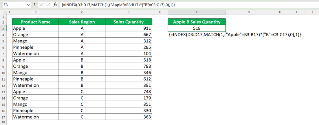
In this example, we try to find the apple sales quantity in Region B. Thus, we have two criteria here to find our data, our product name (apple) and sales region (B).

To find the sales quantity, we use the INDEX MATCH formula writing that we have discussed previously. We pair each of our criteria (apple and B) with its corresponding column (“Product Name” and “Sales Region”) in our MATCH before multiplying the pairings and evaluating the multiplication result with 1. As a result, we get the row position of the sales quantity that fits our criteria (with the “Apple” product name and “B” sales region) and we get the correct result from our INDEX MATCH (518).

Case Sensitive INDEX MATCH: INDEX MATCH EXACT

What about if we want our INDEX MATCH to be case-sensitive? We may have data that is only differentiated by letter cases and we want our INDEX MATCH to recognize that so we can find the right data with it.

For this, we can combine our INDEX MATCH with the EXACT function. The general writing form of the formula resulting from the combination is something like this, assuming that we want to find our data vertically.



We use the EXACT function as an input in our MATCH here.

We input TRUE as the value that we want to find with MATCH. Then, we input an EXACT formula that tries to compare the actual value we want to find the row position of and the column where we want to find that value.

As EXACT is case-sensitive in its comparison process, we will get an array with TRUE and FALSE as its content that already considers the letter cases in the data of the column. TRUE means that the data in the column is the data we want to find and FALSE means it isn’t. This array will then be evaluated by our MATCH to find where the row position of the data with the TRUE value is.

Because of this process in our MATCH, we should get the result we want from our case-sensitive INDEX MATCH!

As an example of the implementation of the case-sensitive INDEX MATCH, see the screenshot below.



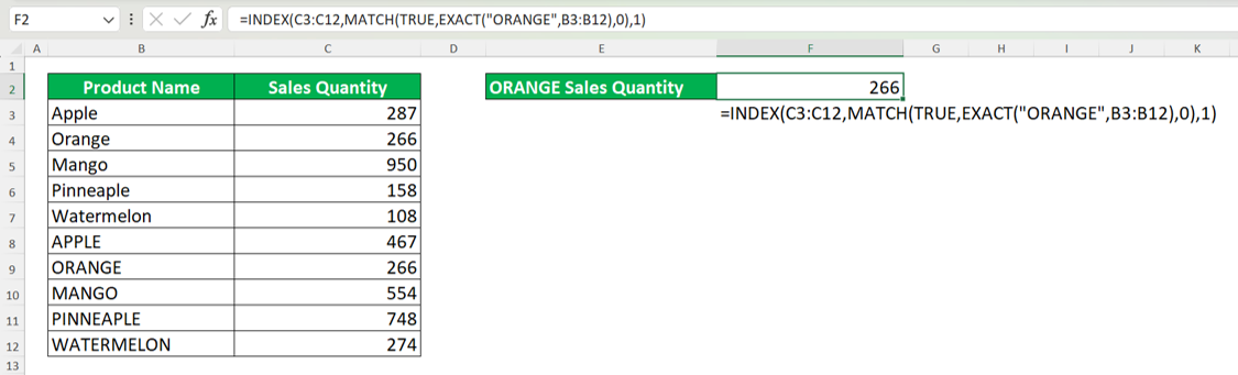
As you can see above, our INDEX MATCH can differentiate the letter cases in our data as it doesn’t return the sales quantity of “Orange”. Instead, it returns the sales quantity of “ORANGE”, the correct one we want to find. That is because we use our TRUE and EXACT formula inputs correctly in our INDEX MATCH!

Exercise

After you have learned completely about INDEX MATCH in Excel, now is the time to do an exercise. This is so you can understand what you have learned from this tutorial more practically.

Download the exercise file below and follow all the instructions. Then, download the answer key file if you have done the exercise and want to check your answers or if you are confused when trying to do the instructions!

Link to the exercise file:
Download here

Instructions

Use INDEX MATCH to do each of the instructions in the appropriate cell according to the instruction number!

1. Find the number value of D!
2. Find the number value of E!
3. Find the number value of A (row) and C (column)!

Link to the answer key file:
Download here

Additional Note

You rarely need the -1 or 1 match type in your MATCH when you use INDEX MATCH. Thus, make sure you input 0 as the last input of your MATCH so you won’t get the wrong result from the INDEX MATCH formula you use.



Related tutorials you may want to learn too: