How to Use Average Excel Formulas
Home >> Excel Tutorials from Compute Expert >> Excel Calculations >> How to Use Average Excel Formulas


In this tutorial, we will discuss completely how to calculate average in excel by using various average excel formulas.
One type of calculation we often do when processing numbers in excel is the average calculation. Therefore, excel provides us with various average formula alternatives to help us do it.
In the next parts of this tutorial, we will discuss in detail the way to use each average excel formula. Each formula has a unique characteristic in its average calculation process and/or result that it produces. If you seriously want to master how to average in excel, then learn this tutorial until the end!
Disclaimer: This post may contain affiliate links from which we earn commission from qualifying purchases/actions at no additional cost for you. Learn more
Want to work faster and easier in Excel? Install and use Excel add-ins! Read this article to know the best Excel add-ins to use according to us!
Table of Contents:
- How to calculate average in excel with the AVERAGE formula
- How to calculate average in excel with 1 criterion: AVERAGEIF
- How to calculate average in excel with more than 1 criterion: AVERAGEIFS
- The criterion writing for average excel formulas AVERAGEIF and AVERAGEIFS
- How to calculate average in excel by including all cells that contain data: AVERAGEA
- How to calculate average in excel with a percentiles consideration: TRIMMEAN
- How to calculate average in excel for filtered numbers: SUBTOTAL
- How to calculate average in excel faster: AutoAverage
- Exercise
- Additional note
How to Calculate Average in Excel with the AVERAGE Formula
If you have experience in calculating average in excel, then most probably the formula you use at that time is AVERAGE.AVERAGE is the basic formula to calculate the average of numbers in excel. By using it, you can get a standard average from the numbers that you have in your worksheet.
In general, here is the writing form of this AVERAGE formula in excel.
=AVERAGE(number1, [number2], …)
The AVERAGE input is all the numbers you want to calculate the average of. You can input them by typing them directly, by using their cell coordinates, or in cell ranges.
Most people usually input a cell range to AVERAGE which contains all the numbers we want to average. If we input more than one number/cell/cell range in AVERAGE, don’t forget to type commas between them!
As a note, if you input cells/cell ranges to AVERAGE, this formula will ignore the cells with non-numeric data.
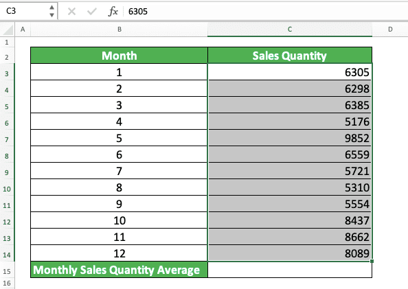
To make it clearer about the use of AVERAGE in excel, take a look at the following example.
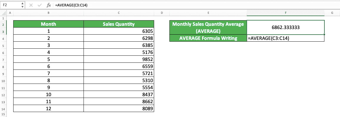
Pretty simple, isn’t it, the excel AVERAGE formula implementation?
In this example, all the numbers we want to average are in a cell range (monthly sales quantity column). Therefore, we just need to input the cell range into AVERAGE to get the average result we need.
The cell range where the monthly sales quantity numbers are is the C3 to C14 cells. Because of that, we input C3:C14 into our AVERAGE formula.
Write AVERAGE, input all the numbers you want to average, and press enter. You will immediately get the average of your numbers!
How to Calculate Average in Excel with 1 Criterion: AVERAGEIF
What if we have a criterion for the data entries with the numbers we want to know the average of? We can use AVERAGEIF to help the calculation process if the criterion is only one.The general writing form of this AVERAGEIF is as follows.
=AVERAGEIF(range, criterion, [number_range])
The AVERAGEIF inputs are the cell range which data we evaluate with our criterion, the criterion, and the number cell range. Note that you can also not input a number cell range. However, the cell range where you evaluate data with your criterion should also be where your numbers are.
If you input different data and number cell ranges, ensure the two cell ranges have the same size and in parallel. This is to make it easier for you to check the result later if needed.
As an implementation example of this AVERAGEIF in excel, see the following example.
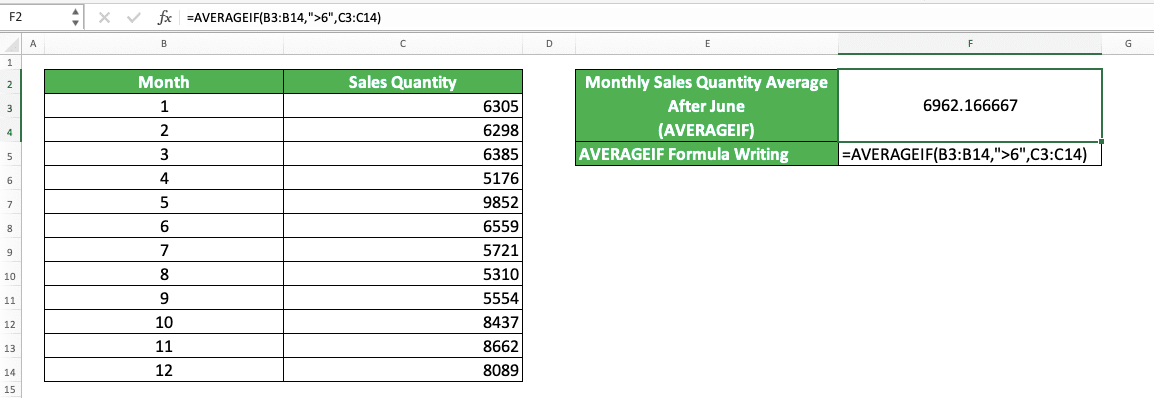
In the AVERAGEIF implementation example, we have a data table of monthly sales quantities and their months. We want to average the monthly sales quantities for months after June.
For that, we input the cell range where the month numbers are as the first cell range input in our AVERAGEIF (the month column cell range, which is B3:B14). We will evaluate this cell range later with our criterion. The criterion itself is the month number which is more than 6 (we write it as “>6” because we want the monthly sales quantities average for the months after June).
The number cell range input is the monthly sales quantity column cell range, which is C3 to C14. The AVERAGEIF writing with these inputs makes AVERAGEIF evaluates the numbers in the month column. The numbers which are more than 6 will pass the criterion.
The monthly sales quantity numbers in parallel with the month numbers above 6 will be included in the average calculation. Because of that, the result becomes 6962.166667, as we can see in the screenshot.
How to Calculate Average in Excel with More than 1 Criterion: AVERAGEIFS
What if we have more than 1 criterion for the data entries which numbers we want to average? For that, we can use the AVERAGEIF sibling formula, which is AVERAGEIFS.The writing form of AVERAGEIFS in excel is as follows.
=AVERAGEIFS(number_range, range1, criterion1, …)
Generally, the AVERAGEIFS inputs are similar to AVERAGEIF. However, you need to input the cell range of the numbers you want to average first.
You must also input the cell ranges of data you want to evaluate with your criterion and their criterion in pairs. One criterion input will only evaluate the data in the cell range we input before the criterion.
Input the pairings of cell range and criterion until you have inputted all your criteria.
Like AVERAGEIF, it is better that all the cell range inputs in your AVERAGEIFS have the same size and in parallel. This is to make it easier for us when we want to check the result later.
As an example of using AVERAGEIFS, take a look at the following screenshot.
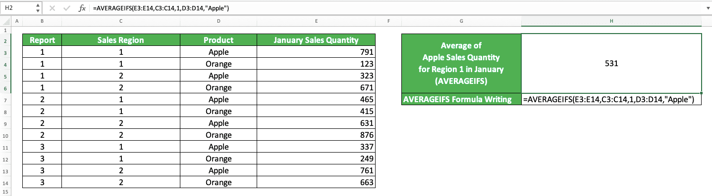
We have the numbers of January sales quantities in the example. The sales quantity numbers have the details of their report, sales region, and product.
We want to calculate the average of January apple sales quantities for region 1. For that, we use AVERAGEIFS by giving inputs based on our calculation needs.
For the number cell range input, we input the monthly sales quantity column cell range. The cell range inputs where we will evaluate data based on our criteria are the region and product columns cell ranges. We input the appropriate criterion (1 and “apple”) after we input each data cell range.
The 1 criterion will evaluate the data in the sales region column and the “apple” criterion will evaluate the product data. All data entries with data that fulfill the criteria will be involved in the AVERAGEIFS average calculation.
As a result, we get a sales quantity average of 531. This is the average of the apple January sales quantities in region 1, the data we look for in the example.
The Criterion Writing for Average Excel Formulas AVERAGEIF and AVERAGEIFS
When using AVERAGEIF and AVERAGEIFS, we must be careful in writing the criteria inputs. The wrong writing can make us get a wrong or even error result.We sometimes might be confused on how to write the criterion we have as the input of AVERAGEIF and AVERAGEIFS. We have known what is the criterion but we don’t know how to write it in excel.
Therefore, Compute Expert will give the criterion writing examples of AVERAGEIF and AVERAGEIFS, with their meanings as well. We hope this can help you in using both formulas according to your data processing needs!
Text (not case-sensitive)
| Criterion Example | Explanation |
|---|---|
| "Jim" | The same as “Jim” |
| “<>Jim” | Not the same as “Jim” |
| “Jim*” | With “Jim” prefix |
| “*jim” | With “jim” suffix |
| “J*m” | “J” prefix and “m” suffix |
| “Jim?” | “Jim” prefix with any one character suffix |
| “?jim” | Any one character prefix with “jim” suffix |
| “J?m” | “J” prefix, any one character, and “m” suffix |
| “Jim~*” | The same as “Jim*” |
| “Jim~?” | The same as “Jim?” |
A bit explanation of the symbols used for the text criterion:
- * = any character in any amount
- ? = any one character
- ~ = used when you want to add a * or ? character for the criterion
Number
| Criterion Example | Explanation |
|---|---|
| 70 | Equal to 70 |
| “>70” | More than 70 |
| “<70” | Less than 70 |
| “>=70” | More than or equal to 70 |
| “<=70” | Less than or equal to 70 |
Date
| Criterion Example | Explanation |
|---|---|
| “>”&DATE(2019,12,3) | Later than 3 December 2019 |
It isn’t recommended to input a date criterion with direct writing (e.g. “>3-12-2019”). The reason is that it can produce a wrong and unexpected result.
Cell coordinate
| Criterion Example | Explanation |
|---|---|
| “>”&B1 | More than the value in B1 |
Empty/non-empty cell
| Criterion Example | Explanation |
|---|---|
| “" | Empty |
| “<>" | Not empty |
How to Calculate Average in Excel by Including All the Cells that Contain Data: AVERAGEA
We may sometimes want to include all the cells that contain data in our average calculation. We want to assume all the cells that contain non-numeric data as zeroes (0).AVERAGE cannot do this because this formula will ignore all the cells that contain non-numeric data in its calculation. To replace AVERAGE, we can use the AVERAGEA formula for this kind of average calculation.
Generally, the AVERAGEA writing is similar to AVERAGE, as you can see below.
=AVERAGEA(data1, [data2], …)
The AVERAGE and AVERAGEA difference is only on the involvement of non-numeric data in its calculation process. AVERAGE will ignore the data while AVERAGEA will involve it by assuming the data as 0.
For an empty cell or data, AVERAGEA will also ignore it just like AVERAGE (except for an excel formula that gives an empty data result (“”). AVERAGEA will involve that by assuming that it has a 0 value).
To make it clearer about AVERAGEA, see the following example.
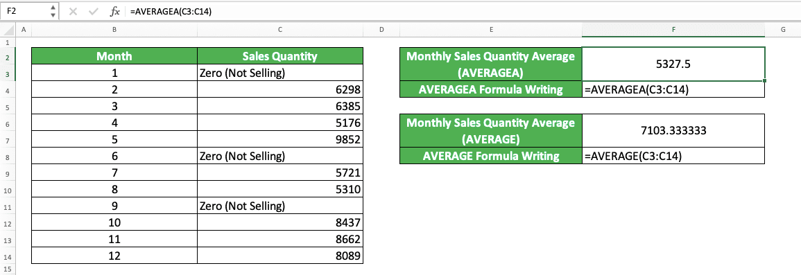
Here, we can see the usage and result of AVERAGEA and its difference with AVERAGE.
In the sales quantity column in the example, there are three texts which represent 0 sales in January, June, and September. With AVERAGEA, we can think of them as 0 because AVERAGEA will assume text data as 0. On the other hand, AVERAGE will ignore them in its calculation.
This difference will cause AVERAGEA to get a smaller average result than AVERAGE. This is because AVERAGEA has zeroes in its calculation while AVERAGE does not.
For the AVERAGEA writing itself, we just input the cell range containing the data you want to average. In this example, the cell range is the cell range of the sales quantity column in the data table.
How to Calculate Average in Excel with a Percentiles Consideration: TRIMMEAN
If we calculate a mean for statistic purposes, we might need to ignore certain top or bottom percentiles of our numbers.The percentiles, for those who don’t know, are the largest or smallest numbers in a group of numbers. If we say 25% top percentiles of numbers, then that includes 25% largest numbers of those numbers.
For the average calculation that considers the percentiles like this, We can use the TRIMMEAN formula in excel.
Generally, the writing form of TRIMMEAN is as follows.
=TRIMMEAN(number_range, percentile_percentage)
The first input of TRIMMEAN is the cell range containing the numbers we want to average. Its second input is the percentage of percentile that we want to ignore in our average calculation from the cell range.
The percentile percentage we input is later divided by two and is distributed equally to top and bottom percentiles. TRIMMEAN won’t involve the top and bottom percentiles which are in this percentage scope in its calculation.
When inputting the percentile percentage, don’t forget to input your number in a percentage (with the percent symbol) or a decimal representing the percentage number. If you input this wrongly, then your TRIMMEAN can produce a #NUM error.
To make it clearer about this TRIMMEAN usage, look at the example below.
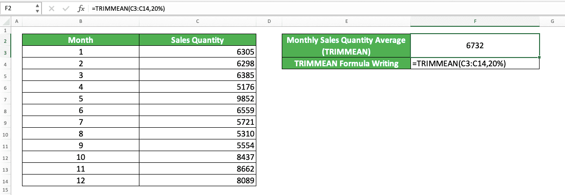
In the example, we want to use TRIMMEAN to average the sales quantities without involving their 10% top and bottom percentiles. Because of that, we input the monthly sales quantity column cell range and a 20% percentage in our TRIMMEAN writing.
TRIMMMEAN will divide the 20% input by 2, resulting in 10% top and bottom percentiles. To determine the number of largest and smallest numbers to “remove”, TRIMMEAN will multiply the 10% with the number of numbers, 12 for the example. This will produce 1.2, which TRIMMEAN will round down to its nearest whole number, which is 1.
That means we will ignore 1 largest number and 1 smallest number in the monthly sales quantities in our average calculation. Because the largest monthly sales quantity is 9,852 (the fifth month) and the smallest is 5,176 (the fourth month), we will ignore these two numbers.
That will make TRIMMEAN produces 6,732 from its average calculation process (the average of the other 10 numbers beside the ones we ignore)!
How to Calculate Average in Excel for Filtered Numbers: SUBTOTAL
What if we want to calculate the average of the numbers that pass the filter we apply in our data table? The AVERAGE formula cannot do it because AVERAGE will keep involving the numbers that don’t pass the filter in its calculation.Is there any particular method that excel provides for this kind of calculation process?
The answer is yes, there is. We can use the SUBTOTAL formula, which excel provides to process filtered data.
Here is the standard formula writing form of SUBTOTAL to average numbers that pass the filter in a data table.
=SUBTOTAL(1/101, filtered_numbers_range)
The 1 or 101 input there is our code to ask SUBTOTAL to average our filtered cell range data. Use 1 if we want to also include the cells we hide manually in the cell range in our calculation. Use 101 if we want to ignore them.
By using SUBTOTAL, we can calculate the average of only the numbers that pass the filter. This is because of the SUBTOTAL nature that ignores the data that doesn’t pass a filter in its calculation.
To make it clearer about this SUBTOTAL usage, take a look at the example below.
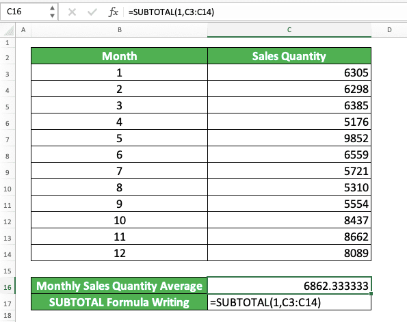
The example shows the SUBTOTAL result if the cell range which becomes its input isn’t filtered yet. The result will be the same as if we use a standard AVERAGE formula.
However, if we filter the data table, then the result will be different as we can see below.
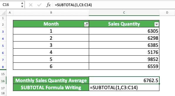
The result of the SUBTOTAL average there is different from the result in the first screenshot. This is because the cell range which becomes the SUBTOTAL input has been filtered in the second screenshot. In the example, we filter with the month basis, which is before July or the month number must be below 7.
If we use AVERAGE, then the calculation result becomes wrong because it keeps calculating the numbers that don’t pass the filter. Because of that, don’t forget to use SUBTOTAL if you have needs like in this example case!
For the SUBTOTAL’s code input part in the example, the result is the same whether we use 1 or 101. This is because there are no data entries we hide manually in the cell range (all of the hidden ones are hidden by the excel filter feature).
How to Calculate Average in Excel Faster: AutoAverage
If your numbers are in one row/column sequence, then you actually can calculate their average fast. Use the AutoAverage feature to do the calculation process for you.If you have used AutoSum before, then this AutoAverage is similar in principles. It is just that the AutoSum sums while the AutoAverage averages the numbers in your number sequence.
You can access this AutoAverage feature by clicking the dropdown of the AutoSum button in your excel Home or Formulas tab.
As an implementation example to make you understand easier, take a look at the following data table.
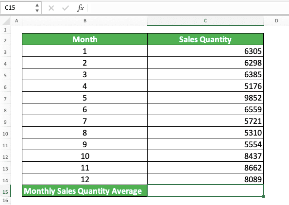
We want to get the average of the numbers in the monthly sales quantity column there. If you use AutoAverage, then you can get the average fast!
To begin using AutoAverage, highlight the number sequence you want to average. Or you can also put your cell cursor one cell outside your number sequence.
Then, click the AutoSum button dropdown in your excel Home or Formulas tab and choose Average. You can see the exact location of this AutoSum button on each tab below.
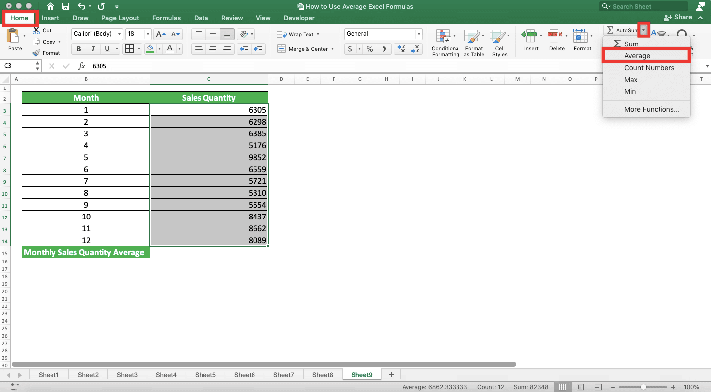
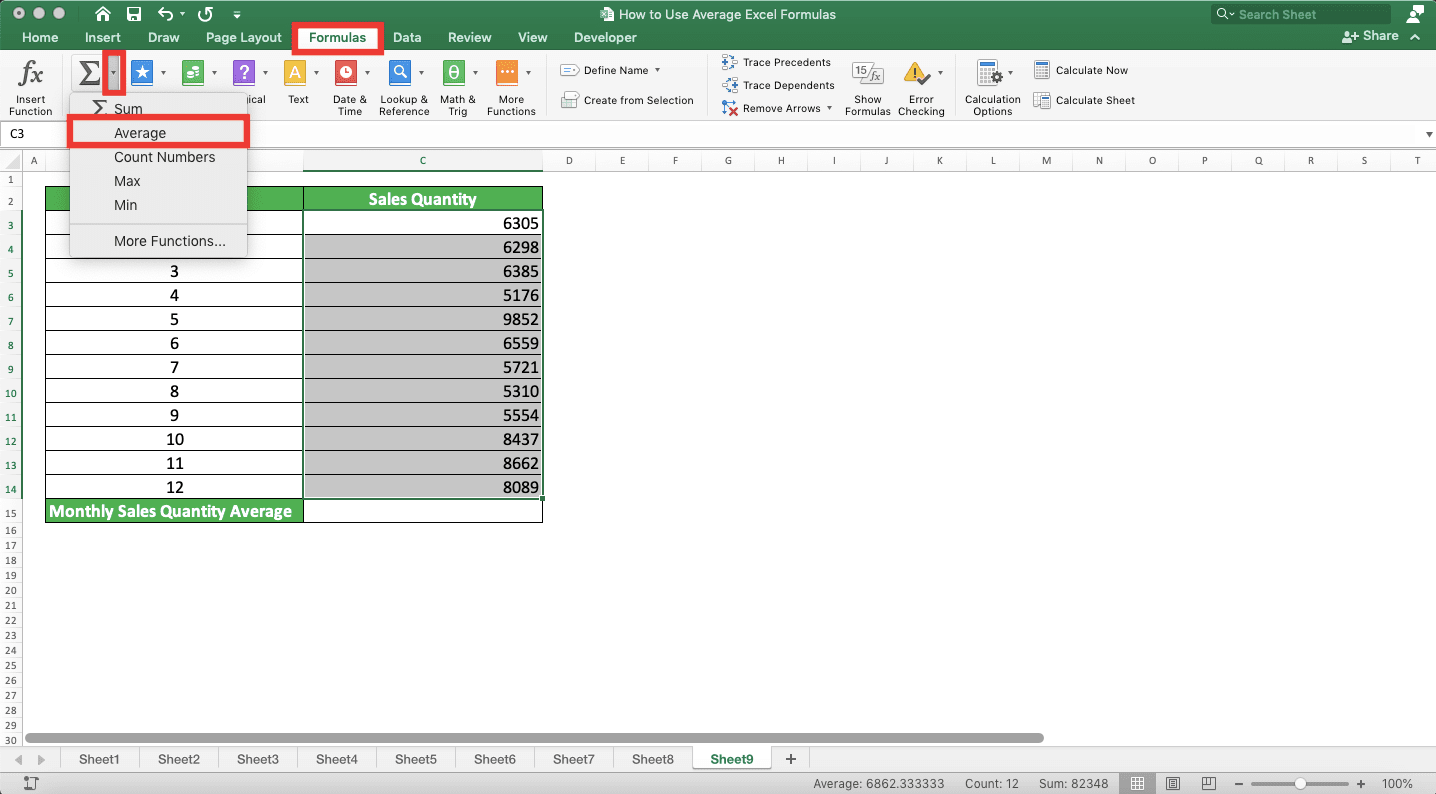
Done! Excel will automatically write the AVERAGE formula for you, one cell outside where your number sequence is. The AVERAGE formula will automatically be inputted with the cell range of your number sequence!
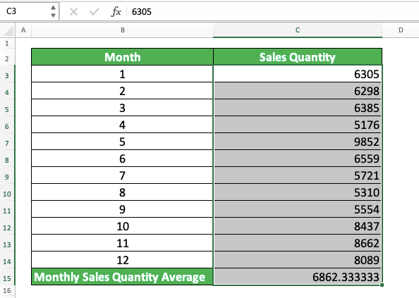
Pretty easy and fast, isn’t it? Use AutoAverage if the numbers you want to average are in a row/column sequence.
Exercise
After you have learned how to use average excel formulas, now let’s do an exercise. The exercise should be done so you can practice your understanding of how to calculate average in excel!Download the exercise file from the following link and answer all the questions. Download the answer key file if you have done the exercise and sure about your answers!
Link to the exercise file:
Download here
Questions
- What is the average number of students for all classes?
- What is the average number of students in class C? Use AVERAGEIF to answer!
- What is the average number of students in classes 1 and 3 with code D? Use AVERAGEIFS to answer!
Link to the answer key file:
Download here
Additional Note
After calculating the average, probably you want to label your data entries based on their number compared with the average. For that, you need to use the IF formula. Learn how to use this formula if you haven’t understood it in this Compute Expert tutorial!Related tutorials for you to learn: