How to Use IF Formula/Function in Excel

In this tutorial, you will learn how to use the IF formula in excel.

IF is one of the most often used formulas in excel. The result you get from IF is based on a certain logic condition evaluation process. If the condition is true, then it will give a result and if false, then it will give another result.

If you haven’t understood or want to know deeper about this formula, then you have come to the right place! After learning the contents of this tutorial, you should be able to use the IF function in excel optimally.

Disclaimer: This post may contain affiliate links from which we earn commission from qualifying purchases/actions at no additional cost for you. Learn more

Want to work faster and easier in Excel? Install and use Excel add-ins! Read this article to know the best Excel add-ins to use according to us!

IF Formula Definition

IF is a formula that can give a result based on a specific logical test.

There are two possible results from that test, TRUE or FALSE. IF will give us a result based on this TRUE or FALSE logic value.

IF Function Usefulness

IF can give us a result according to the logical test process that we give as an input in it.

IF Result

IF result is particular data/process based on whether our logic condition input has a true or false value.

Excel Version from Which We Can Start to Use IF

We can start to use IF since excel 2003.

The Way to Write It and Its Input

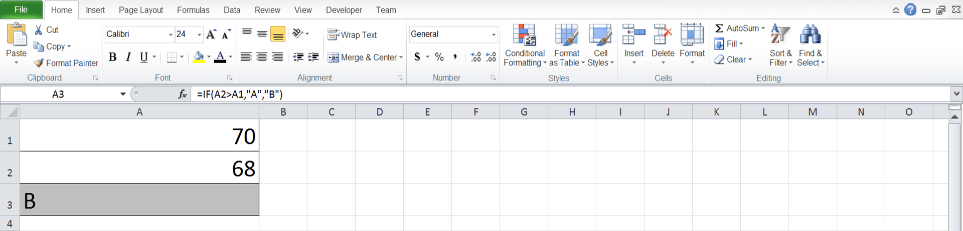
Here is the general form of the IF writing in excel.



And here is the explanation of the inputs.

• logical_test = the logic condition you want to evaluate using IF. The evaluation result will determine the result you get from your IF
• [value_if_true] = optional. The IF result if the logic condition you input is true. If you don’t input here, then the result will be a TRUE logic value
• [value_if_false] = optional. The IF result if the logic condition you input is false. If you don’t input here, then the result will be a FALSE logic value

Logic Operators

When writing an IF in excel, we usually use one of the logic operators available when we input its logic condition. The logic operator will compare the two data we input in each of its sides. It has an important role in determining whether your logic condition as true or false.



Generally, there are 5 logic operators we can use in excel. You can see those five operators and their meaning in the table below.

Logic Operator	Meaning
=	Equal to
<	Less than
>	More than
<=	Less than or equal to
>=	More than or equal to

Don’t be wrong in choosing your logic operator when you use an IF!

IF Formula Example 1: Pass and Fail

To make you understand about the IF formula in excel, we will give three examples of its implementation. The first example is about the pass or fail of students based on their test score numbers.

You can see the IF implementation for this first example in the screenshot below.



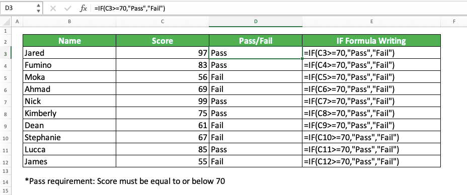
In the example, we can see how IF helps us determine the pass or fail labels of all students in the list. To use IF, we must input the passing requirement, which is the test score must be equal to/more than 70. See the way to input this requirement in IF in the screenshot.

Moreover, we shouldn’t forget to input the word “Pass” if the condition is true and “Fail” if the condition is false.

By giving its inputs correctly, IF gives us the correct passing labels for each student fast and easily.

IF Formula Example 2: Discount Lookup in Excel Using IF

The second example of the IF implementation is about finding the right discount level in excel. We usually need this when we have several discount levels depending on the total payment value.

We can see the example of the IF implementation to find this discount level below.



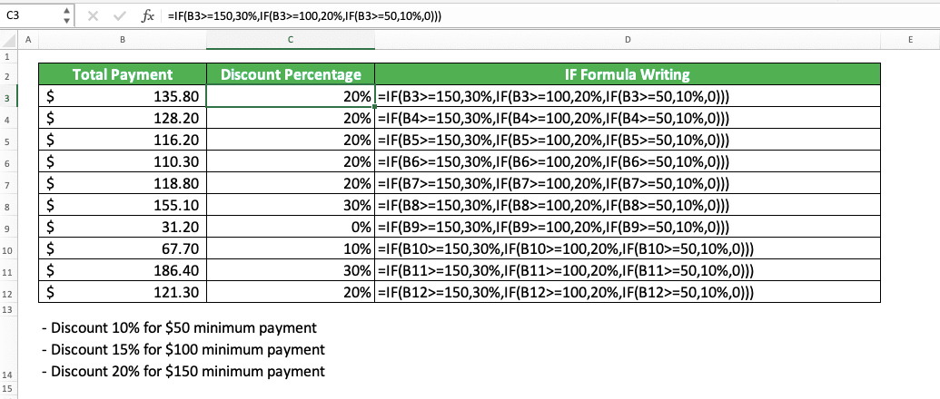
To find the discount level based on the total payment value, we use an IF form called nested IFs. We use this because there are more than one logic conditions we need to test. We need to test all of them to get the right discount percentage for each total payment value.

In the example’s IF writing, we input the conditions in reverse so we don’t get the wrong result (if we input >=500000 first, then it will also be TRUE if the value is more than 1 or 1.5 million). We input the condition for the >1.5 million first followed by >1 million and >500000. Each condition has its own IF writing as you can see in the screenshot.

We input each IF writing in the previous IF in its FALSE result input. This is why we often call this nested IFs because the way to write the IFs is “nested”. If the first IF is wrong, then we go to the second IF. If it is wrong too, then we go to the third one, and so on.

After we input the conditions, we input the discount percentage we want if the condition is true. Last but not least, we also input the discount percentage if all the conditions we input are false (in the example, that means if the total payment value is lower than 500,000).

Write the IF formula and give the IF inputs correctly. You will get the discount percentage for each of the total payment values immediately!

IF Formula Example 3: Employees’ Attendance

The last IF implementation example here is the IF to help to process the employees’ attendance data. To understand this implementation, see the following screenshot.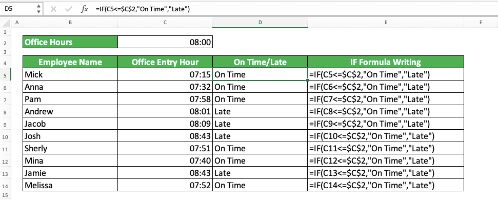



In this example, we can see how IF determines whether the employees are late/not based on their office entry hours. IF can do this by comparing the employees’ entry hours with the office hour.

We give the logic condition input that the entry hour must be less than or equal to the office hour. If true, then we will label the employee “On Time” and if not, then we will label the employee “Late”. All these inputs produce the result we want.



If you are confused about the $ symbol in the C2 cell coordinate input, it is an absolute reference symbols in excel. By using it, the cell coordinate won’t move when we copy the formula to other cells (we need the $ symbols because the office hour reference is only on one cell for all the IFs, which is C2. With those symbols, we can copy our IF formula much easier and faster).

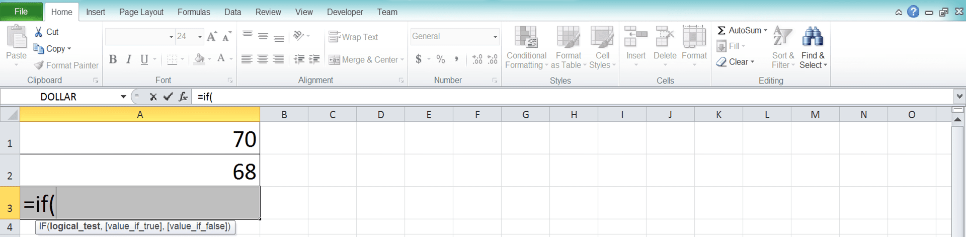
Writing Steps

What are the steps to write IF in excel from the beginning until the end? Here are the details for you.

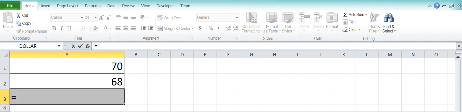
1. Type an equal sign ( = ) in the cell where you want to put the IF result
   
   
   
   
2. Type IF (can be with large and small letters) and an open bracket sign after =
   
   
   
   
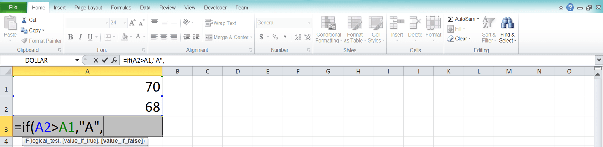
3. Input the logic condition which you want to evaluate to determine your IF result. Then, type a comma sign ( , )
   
   
   
   
4. Input the IF result if the logic condition is true. After that, type a comma sign
   
   
   
   
5. Input the IF result if the logic condition is false
   
   
   
   
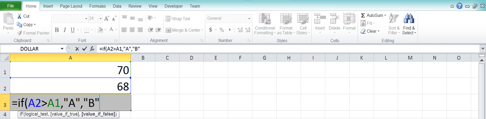
6. Type close bracket sign
   
   
   
   
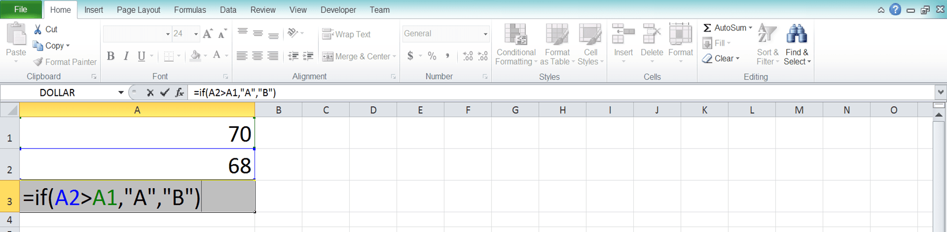
7. Press Enter
8. The process is done!
   
   
   
   

Factors that Can Cause the IF Formula to Not Work/Produce an Error/Wrong Result

Having some troubles when you want to get a result from your IF in excel? Probably you get a result that is unexpected in a bad way.

Of course, various factors can cause this. However, the main factors that usually make an IF result wrong or error is as follows.

• You don’t input a complete logic condition and/or you don’t put a logic operator in it
• You have text for the result inputs in your IF and you don’t give quotes as you type them directly
• If you use nested IFs, then you might wrongly put your IF in the previous IF

Check your IF formula writing again if its result confuses you and make sure you don’t do the mistakes above!

Single IF

If you often use excel or read excel writings, then you might have heard the single IF term. What is a single IF? It is the IF formula writing consisting of only one IF.

Because you can have more than one logic conditions, then the IF we use can also be more than one. However, if we use a single IF, then the logic condition we need to test is only one. Because of that, we only need to use one IF in our formula writing.

In general, here is the writing form of a single IF.



And here is its implementation example in excel.



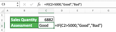
We can see there how we do a single IF formula writing and the result we get from it. A single IF gives a result depending on the inputs we give in it.

Double IFs

What about the one we call double IFs? Double IFs is the IF formula writing where there is an IF in another IF. The writing of the IF is usually in the result input part of its the other IF.

Generally, here is the writing form of double IFs in excel.



This writing will give its result from the IF inputs in the other IF. If you don’t need it, then you can replace one of the inside IFs with other things.

As an implementation example of the double IFs, take a look at the following screenshot.



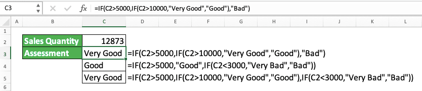
In the double IFs example, we can see how IF in another IF affects the result we get. We add a criterion in the inside IFs besides the one we give in the outer IF.

There are 3 forms of double IFs we can use as seen in the example. The result we get depends on the process we run in the form we use. The IF inside another IF makes excel needs to read logic conditions twice before it gives us a result.

We can read the formula process like an “and” to fulfill the two IFs conditions. For example, see the process that happens in the first double IFs writing above.

If the sales quantity is more than 5000 and more than 10000, then the result will be “Very Good”. If more than 5000 but less than 10000, then the result will be “Good” only. If it cannot fulfill those two criteria, then the result will be “Bad”.

A similar process like this also happens in the other two double IFs writings in the example.

Nested IFs

There is one more IF formula form we often use in excel. We call this one nested IFs.

Nested IFs is the writing form in which we place an IF in the FALSE result input part of another IF. We can do this several times until we form some phases of IFs.

In general, here is the writing form of nested IFs in excel.



In the writing form like this, excel will evaluate logic conditions continuously until it finds a true condition. From there, our nested IFs writing will take its final result.

In the nested IFs, we keep writing our IF until we have inputted all the logic conditions and results we need. We can use a maximum of 64 IFs in the same writing.

To make it clearer about this nested IFs implementation, see the example in the screenshot below.



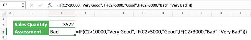
In the screenshot, we can see exactly the writing form and result of nested IFs in excel. We get “Bad” there because the IF condition that has this result produces TRUE.

In nested IFs, you need to determine the logic condition you want to evaluate early so you can type it first. Determine wisely so you don’t get the wrong result from your nested IFs.

Like in the example, we evaluate the condition where the sales quantity is more than 10000 first. This is because if we start with a smaller number, then IF won’t evaluate the logic condition of more than 10000 (because sales quantity more than 10000 is more than 3000 or 5000 too).

Moreover, don’t forget to input the result if all the logic conditions we input in our IFs are FALSE. In the example, if the sales quantity doesn’t fulfill all the IFs requirements, then it must have a very low number (less than 3000). This makes us label the quantity with the words “Very Bad”.



If you want to learn further about the nested IFs implementation in excel, then you can visit this tutorial.

IF Formula Combination We Often Use 1: IF AND OR NOT (IF With More Than 1 Logic Conditions)

What if we want to evaluate more than one logic condition simultaneously in one IF? Or, probably, we want to reverse TRUE to FALSE or otherwise in our IF’s logic condition part?

We can do these things by combining our IFs with AND, OR, or NOT formulas.

For you who don’t know these formulas, here is a brief explanation of those three’s functions.

• AND: evaluates more than one logic conditions/values and gives TRUE if all the logic conditions/values are TRUE
• OR: evaluates more than one logic conditions/values and gives TRUE if at least one of them is TRUE
• NOT: reverses TRUE to FALSE and FALSE to TRUE

Here are the general writing forms of the combination between IF and each of the three formulas.

IF AND:



IF OR:



IF NOT:



Those three formulas, AND, OR, and NOT, focus on the logic condition input of your IF. If we use AND or OR, then gives all the logic conditions you want to combine in it, separated by comma signs.

Don’t choose AND or OR wrongly when you combine the logic conditions in your IF. If you choose wrongly, then you will get the wrong IF result too.

We can also combine AND, OR, and NOT in one IF if you need it. Like, maybe, when you want to reverse the logic value you get from your OR. You can do it by writing NOT that envelopes OR like this: NOT(OR(logical_test_1, logical_test_2))

To make it clearer about the use of IF with those three formulas, here is an example of it in excel.



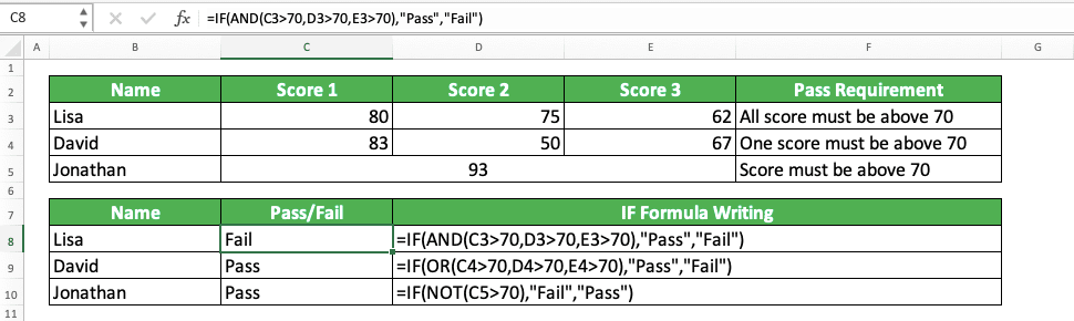
In the above example, we can see the writing and result of the IF combination with AND, OR, and NOT. We can also see the function of each formula in the IF there.

AND will give TRUE to IF if all of its logic conditions/values inputs are TRUE. Because of that, it fits the requirement to get the pass/fail result from Lisa there.

We can also see the way to write the formula to get Lisa’s result in the screenshot. We input the condition for each score comparison with 70, separated by comma signs.

Because there is one score below 70 (the third score, 62), AND gives FALSE for the IF. Because of that, IF gives us its FALSE result there, which is the “Fail” label.

For the second case (the pass/fail for David), we use OR because just one of the conditions there needs to be TRUE. Like AND, we give the inputs of all the scores compared with the passing score, 70, in our OR.



Because there is at least one score that fulfills the requirement (first score, 83), OR gives TRUE to the IF. Because of that, IF produces its TRUE result, which is the “Pass” label.

The case of pass/fail for Jonathan is an implementation example of NOT. Inside NOT in the IF, we input the condition of the score needs to be more than 70. The TRUE result in the IF there is “Fail”.

Because Jonathan’s score is more than 70, then the logic condition we input produces TRUE. But because we use NOT, this result is reversed to FALSE. The FALSE makes the iF gives its FALSE result to us, which is the “Pass” label.

IF Formula Combination We Often Use 2: IF ISERROR, ISNA, IS… (IF with Data Type Testing)

Have you ever used an IS formula in excel for your data processing?

IS formulas are the formula that gives us TRUE or FALSE based on the data type we give as their input. You can see the members of the IS formulas in excel and a bit of explanation of their functions below.

• ISBLANK: gives TRUE if its input is a blank data/cell
• ISERR: gives TRUE if its input is an error besides #N/A
• ISERROR: gives TRUE if its input is an error
• ISLOGICAL: gives TRUE if its input is a logic value (TRUE/FALSE)
• ISNA: gives TRUE if its input is a #N/A error
• ISNONTEXT: gives TRUE if its input is non-text data (also gives TRUE for a blank data/cell)
• ISNUMBER: gives TRUE if its input is a number
• ISEVEN: gives TRUE if its input is an even number
• ISODD: gives TRUE if its input is an odd number
• ISREF: gives TRUE if its input is a reference
• ISTEXT: gives TRUE if its input is a text
• ISFORMULA: gives TRUE if its input is a formula

The writing form for all the IS formulas is similar. We input our data to the IS formula we use to get a TRUE/FALSE result.

If needed, we can also use IS with an IF. When we need to determine our IF result according to our data type, we can use the help of IS formulas.

Generally, here is the writing form of the combination between IS formulas and IF.



As you may guess, because it produces TRUE/FALSE, we usually put an IS formula in the IF’s logic condition part. Input the IS with the data we want to evaluate the type of to get the result we want.

To better understand how to use this combination, here is its implementation example in excel.



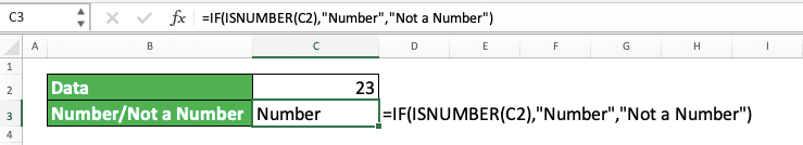
The example above combines one of the IS formulas, ISNUMBER, with IF. This is because we need to test whether our data is a number or not.

As you can see, you just need to type ISNUMBER and its data input in the IF. If you want to use another IS to give a logic condition input in your IF, then the writing is similar (just need to change ISNUMBER with the IS formula name you want to use)

By using ISNUMBER there, we can get our TRUE/FALSE result after checking our data type (whether it is a number or not). From there, we get the result we need in the example!

IF Formula Combination We Often Use 3: IF VLOOKUP

Sometimes, maybe we need to get an IF result based on the data lookup process we do in a cell range. If we find data like this, then the result is this and if we find that, then we get another result.

How we can do that in excel? One of the ways is by combining the IF and VLOOKUP formulas in one writing.

If you often use excel, then you most probably have used VLOOKUP. It is one of the formulas we most often use in excel. It has a function to find data vertically in a cell range.

If you want to combine it with IF with the purpose as above, then the writing form is generally like this.



We put the VLOOKUP in our IF’s logic condition input part. We decide the logic operator we put after the VLOOKUP (the = symbol after the VLOOKUP writing above) depending on what kind of logic condition we want to evaluate.

To make this explanation of the IF and VLOOKUP combination clearer, here is its implementation example.



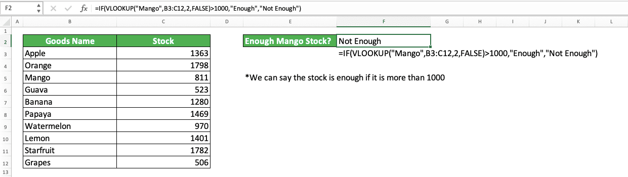
We can see in the example how we base our IF result on the VLOOKUP result we get.

Here, we want to make sure the mango stock is sufficient by finding the stock number first on the table. We determine the stock sufficiency by checking whether the mango stock quantity is above 1000.

If it is above 1000, then we give an “Enough” label and if not, then we give a “Not Enough” label. We find the stock number using VLOOKUP and give the label using IF, based on the VLOOKUP result.

What if we want to use VLOOKUP in the TRUE and/or FALSE results of our IF? Of course, we just need to put the VLOOKUP in the appropriate parts of the IF.

Generally, here is the IF and VLOOKUP combination writing form for that purpose.



In the writing, we can see that we base which VLOOKUP we use on the logic condition evaluation result. If TRUE, then we use the first VLOOKUP and if FALSE, then we use another VLOOKUP.

If you don’t need it, then you can replace one of the VLOOKUPs with another IF result you want.

To understand this IF VLOOKUP combination clearer, here is its implementation example in excel.



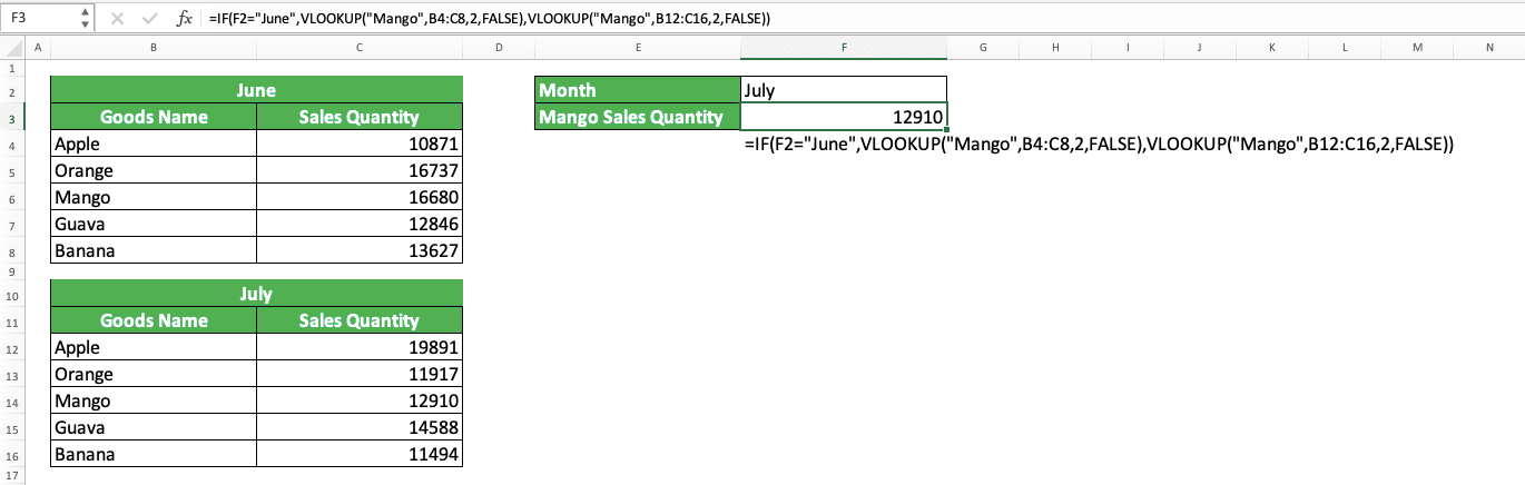
In the example, we use IF VLOOKUP to look for the sales quantity data we need. There are two reference tables and we choose one table based on the month we need.

In the IF there, we write if the month cell value is June, then we use VLOOKUP on the June table. If the value isn’t June (which means it is July in the example), then we use VLOOKUP to look for the quantity data in the July table.

The IF and VLOOKUP combination helps us get the data lookup result we need!

If what you need is to understand the use of IF in VLOOKUP, then visit our VLOOKUP tutorial that discusses it!

IF Formula Combination We Often Use 4: IF LEFT MID RIGHT

If we want an IF logic condition that uses a part of a text, then we can use LEFT/MID/RIGHT. Input their writings in our IF correctly to get the result we want.

You obviously need to know what are the functions of LEFT/MID/RIGHT in excel first before using one of them. Briefly, we can explain the functions of those three formulas as follow.

• LEFT: gets a part of a text from the left side of the text
• MID: gets a part of a text. You can determine the starting position from where you want to get the text part
• RIGHT: gets a part of a text from the right side of the text

As you can see, the main difference between those formulas is in the position from where it gets the text part. Use the formula which is appropriate to your data processing needs in your IF writing.

The following will give the general writing form of the IF combination with each of those three formulas,

IF LEFT:



IF RIGHT:



IF MID:



Input the text and the number of characters you want to get from that text in your LEFT/RIGHT/MID. For MID, don’t forget to input the position where you want to start getting this part of the text.

You can change the logic operator after you write LEFT/RIGHT/MID (= symbol above) depending on your need. Don’t forget to input the TRUE and FALSE results correctly too so you can get the IF results you want.



To make it easier for you to understand the combination, here is its implementation example in excel.



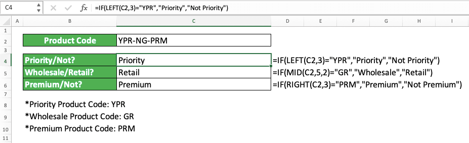
From the example above, we want to translate parts of the product code. Each part has its own meaning which can give partial information about the product.

We can translate them by using the combination of IF and LEFT/MID/RIGHT. We can separate the part we need by using one of those three formulas first. After getting the part of the code, we can translate it using IF.

The number of meanings of each code part, which is only 2, helps to make the work in the example easier. If there are more than 2 meanings, then we need to use nested IFs to translate them.

We have discussed the use of LEFT/MID/RIGHT in the logic condition input part of IF. But, what about the use of them in the TRUE/FALSE results input part of our IF?

Here is the implementation example of this in excel.



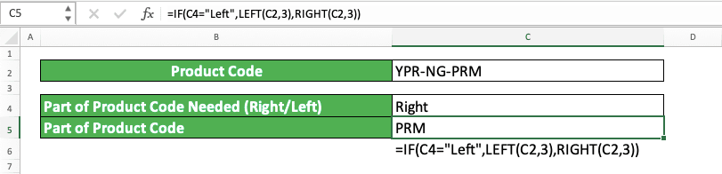
In the example, we will take a part of the product code depending on the cell value, “Left” or “Right”. If “Left”, then we take the left part of the code and if “Right”, then we take the right part.

We can do this by writing an IF and input the LEFT and RIGHT formulas in the correct IF input parts. Here, we input the logic condition if the cell value is “Left”.

If “Left”, then we use LEFT and if not “Left” (which means “Right” in the example), then we use RIGHT. Give the right inputs to the IF to get the IF result you need!

IF Date Formula (DATEDIF)

In processing dates, sometimes we might want to calculate the difference between 2 dates. That difference can be on the days, months, or years, depending on the data processing needs we have.

If we use a normal subtraction calculation in excel, then we will only get the whole days’ difference. What if we want the months or years’ difference? Or the days’ difference without considering the months and/or years?

We can do this by using the if date formula variant, which is DATEDIF.

Generally, here is the writing format of DATEDIF in excel.



In writing DATEDIF, we input two dates we want to calculate the difference on. We start its input by placing the earlier date first before inputting the later date.

Last but not least, we give the unit which represents the difference we want from those two dates.

Here are the unit inputs we can give to DATEDIF and the explanation of the difference we can calculate using them.

Unit	Calculate the Difference of	Additional Note
Y	year	-
M	year	includes year
D	day	includes month and year
MD	day	excludes month and year
YM	month	excludes year
YD	day	excludes year

The meaning of includes/excludes in the additional note is whether we consider the month and/or year numbers when calculating.

For example, let’s say we want to calculate the difference between 2 January 2021 and 3 February 2021. If we use the MD unit, then the difference is 1 day (ignoring the month and year numbers differences). However, if we use the D unit, then the difference is 32 days (considering the month and year numbers differences too then translating the differences to add to the days’ difference).

To make it clearer about DATEDIF usage and result, here is its implementation example.



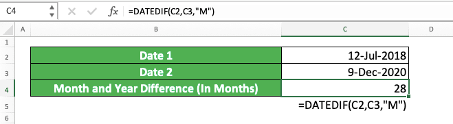
Here, we want to calculate the month difference between the two dates by considering the year difference too. We can do this calculation easily using DATEDIF.

The unit we use in the DATEDIF here is “M”, which calculates the months’ difference by considering the year numbers. By using the correct DATEDIF inputs, we can immediately get the months’ difference we want!

If you want to know more about DATEDIF, then please visit the Compute Expert tutorial which discusses it specifically here.

Other IF-Like Variants (SUMIF, SUMIFS, AVERAGEIF, AVERAGEIFS, COUNTIF, COUNTIFS, IFERROR, IFNA)

In excel, we can also use several formulas that help us calculate based on specific criteria. If the data fulfill the criteria, then we calculate it and if not, then we don’t. We can assume these formulas as the IF-like formulas which can help us process our number data easier.

There are also other two formulas with IF-like functions to help us to anticipate errors in excel. Those two formulas are IFERROR and IFNA.



Generally, here is the explanation of the calculation and error anticipation formulas with the IF-like functions. There are also their Compute Expert tutorial links if you want to learn more about some of those formulas!

• SUMIF: sums numbers from the data entries that fulfill one specific criterion
• SUMIFS: sums numbers from the data entries that fulfill specific criteria (can be one or more than one)
• AVERAGEIF: averages numbers from the data entries that fulfill one specific criterion
• AVERAGEIFS: averages numbers from the data entries that fulfill specific criteria (can be one or more than one)
• COUNTIF: counts the amount of data that fulfill one specific criterion
• COUNTIFS: counts the amount of data entries that fulfill specific criteria (can be one or more than one)
• IFERROR: anticipates an error by giving an alternative value if the error does happen
• IFNA: anticipates a #N/A error by giving an alternative value if the #N/A error does happen

Quite many formulas, isn’t it? If you want to use the IF function for calculation or error anticipation objectives, then these formulas can definitely help you.

Exercise

After learning how to use the IF formula in excel, now let’s do an exercise. This is so you can understand more about the IF implementation in excel.

Download the exercise file through the link below and answer all the questions. Download the answer key file if you have done the exercise and want to check your answer. Or probably when you are confused about how to answer the question!

Link to the exercise file:
Download here

Questions

Are the sales targets of Niko, Cathy, and Acong achieved? Use IF to answer it with the “Achieved” or “Not Achieved” label!

Link to the answer key file:
Download here

Additional Note

If you need it, then you can also type a TRUE or FALSE logic value directly in your IF. Excel will automatically convert a TRUE or FALSE text you type into a logic value.



Related tutorials you should learn too: