How to Use SUMIF Excel Formula: Function, Example, and Writing Steps
Home >> Excel Tutorials from Compute Expert >> Excel Formulas List >> How to Use SUMIF Excel Formula: Function, Example, and Writing Steps


In this tutorial, you will learn completely about the SUMIF excel formula, from its basic principles to its advanced use.
SUMIF is one of various sum formulas you can use in excel. You can often take advantage of its function, depending on the kind of number processing you have to do in excel.
Master this formula here so you can utilize it optimally for your data processing work!
Disclaimer: This post may contain affiliate links from which we earn commission from qualifying purchases/actions at no additional cost for you. Learn more
Want to work faster and easier in Excel? Install and use Excel add-ins! Read this article to know the best Excel add-ins to use according to us!
Table of Contents:
- SUMIF function in excel
- SUMIF result
- Excel version from which SUMIF can be used
- The way to write it and its input
- Example of its usage and result
- Criterion writing in SUMIF
- Writing steps
- Main reasons why your SUMIF produces an error/wrong result
- Horizontal SUMIF
- Sum numbers with a cell/font color criterion: XLTools
- SUMIF with OR criteria
- SUMIF with AND criteria: SUMIFS
- SUMIF with the criterion in a separate table: SUMIF VLOOKUP/SUMIF INDEX MATCH
- SUMIF for multiple number columns
- Exercise
- Additional note
SUMIF Function in Excel
We can use SUMIF to sum the numbers from data entries that fit our criterion.SUMIF Result
The result of SUMIF is the total of numbers from data entries that fit our criterion.Excel Version from Which SUMIF can be Used
We can use SUMIF since excel version 2003.The Way to Write It and Its Input
Generally, you should write SUMIF like this in your cell in excel.
= SUMIF ( data_range, criterion, [numbers_range] )
The explanation of the inputs there is as follows:
- data_range = the cell range that contains the data you want to evaluate with your criterion
- criterion = the criterion that determines whether we should include a data entry number in our sum process or not
- numbers_range = optional. The cell range that contains the data entries numbers we will sum if the data entries meet the criterion. If you don’t give input here, then excel will sum the numbers in the data range
If you input a numbers range, ensure the cell range is in parallel and the same size as the data range. This is so you can check the SUMIF result much easier later when you need to.
Example of Its Usage and Result
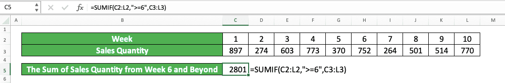
Here is a screenshot that shows the example of the SUMIF usage and result in excel.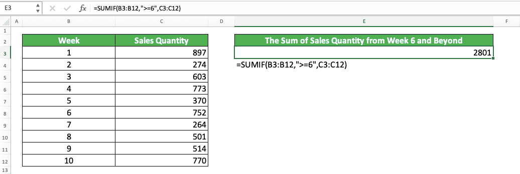
In this example, we try to sum the sales quantities from week 6 and beyond. To do that, we can use SUMIF to help us.
As the week and the sales quantity data are different, we input two cell ranges in our SUMIF. The week column becomes the data range and the sales quantity column becomes the numbers range.
As seen in the formula in the example, we input those cell ranges in parallel and at the same size. Thus, it will be easier for us to see the numbers that contribute to the sum result.
As for the criterion, because the week data are already in numbers, we input a number criterion there. More than week 6 here translates to “>=6” in the criterion writing in excel.
If you want to see other criterion writings you can use in SUMIF, read the next part of the tutorial below.
Criterion Writing in SUMIF
If you want to get the correct result from SUMIF, then you need to input your criterion correctly. This is to make sure that the data in your data range will be evaluated as you prefer them to.How to write the criterion you want in SUMIF? There are different kinds of writing you should use depending on the criterion you have. Here are the criterion writing examples you can refer to and their meanings.
Text (not case-sensitive)
| Criterion Example | Explanation |
|---|---|
| "Jim" | The same as “Jim” |
| “<>Jim” | Not the same as “Jim” |
| “Jim*” | With “Jim” prefix |
| “*jim” | With “jim” suffix |
| “J*m” | “J” prefix and “m” suffix |
| “Jim?” | “Jim” prefix with any one character suffix |
| “?jim” | Any one character prefix with “jim” suffix |
| “J?m” | “J” prefix, any one character, and “m” suffix |
| “Jim~*” | The same as “Jim*” |
| “Jim~?” | The same as “Jim?” |
A bit explanation of the symbols we can use for the text criterion:
- * = any character with any amount
- ? = any one character
- ~ = use it when you want to add a literal * or ? character for the criterion
Number
| Criterion Example | Explanation |
|---|---|
| 70 | Equal to 70 |
| “>70” | More than 70 |
| “<70” | Less than 70 |
| “>=70” | More than or equal to 70 |
| “<=70” | Less than or equal to 70 |
Date
| Criterion Example | Explanation |
|---|---|
| “>”&DATE(2019,12,3) | Later than 3 December 2019 |
It isn’t recommended to input a date criterion with direct writing (e.g. “>3-12-2019”). This can produce a wrong and unexpected result.
Cell coordinate
| Criterion Example | Explanation |
|---|---|
| “>”&B1 | More than the value in B1 |
Empty/non-empty cell
| Criterion Example | Explanation |
|---|---|
| “" | Empty |
| “<>" | Not empty |
Writing Steps
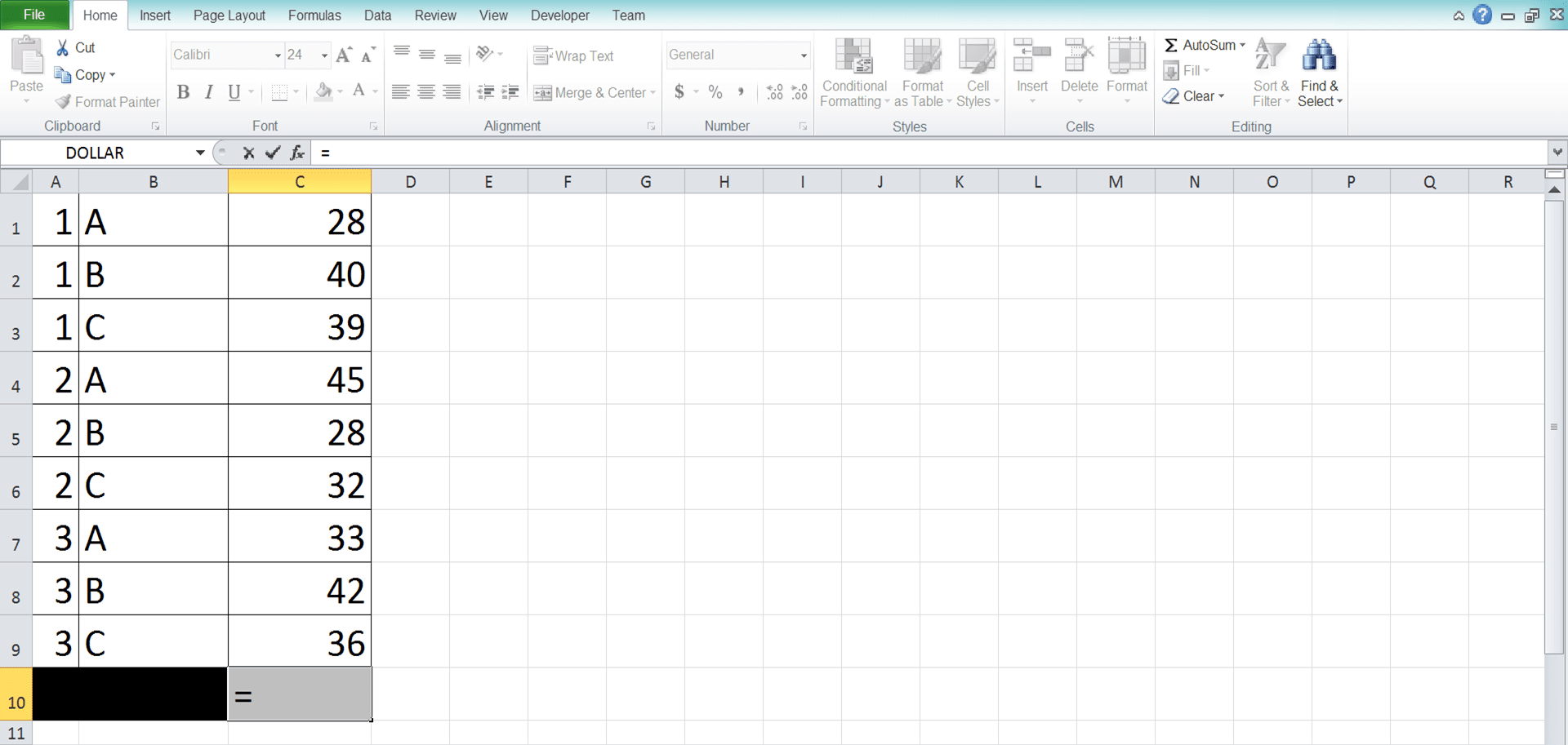
After learning the SUMIF implementation example and its criterion writing, now let’s learn its detailed writing steps. We give the steps explanation here with example screenshots to help you understand it much easier.-
Type an equal sign ( = ) in the cell where you want to put the SUMIF result in
-
Type SUMIF (can be with large and small letters) and an open bracket sign after =
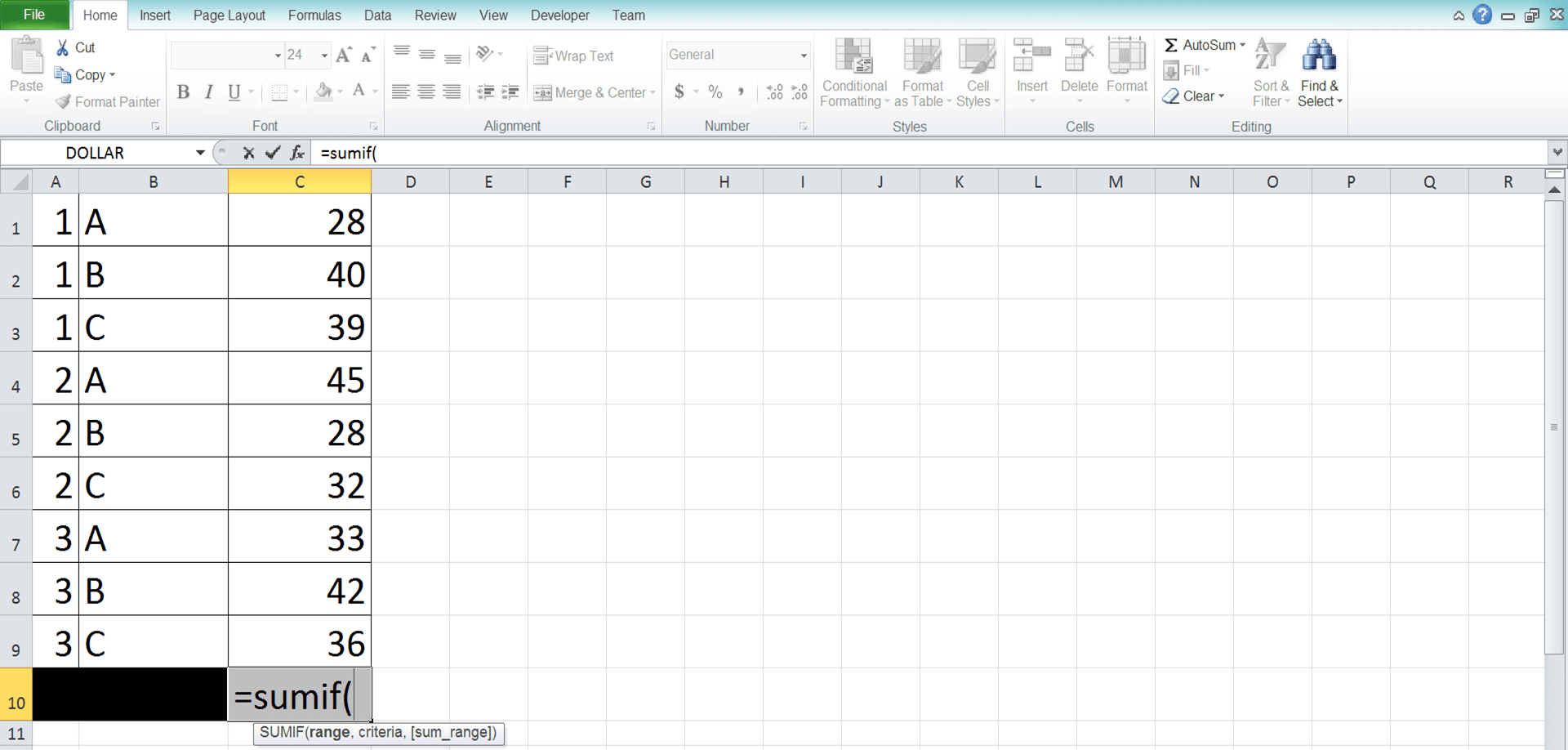
-
Input the data range where your criterion will evaluate your data. This data range can also be the numbers range where SUMIF will sum your numbers if they are the same. After that, type a comma sign ( , )

-
Input your criterion then type a comma sign
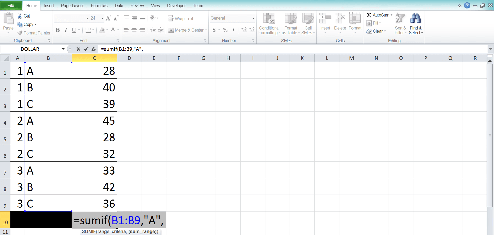
-
Optional: If your data range is different than your numbers range, then input your numbers range here. The numbers range should be inline vertically/horizontally with the data range. They must also have the same number of cells
-
Type a close bracket sign

- Press Enter
-
The process is done!

Main Reasons Why Your SUMIF Produces a Wrong/Error Result
Got an error or wrong result from your SUMIF?Many factors can cause that. However, one of these factors is probably the cause of the problem most of the time.
- You don’t input the correct data and number cell ranges. Take a look again at your cell range inputs and make sure that you have already inputted the right ones. Maybe you give the wrong cell coordinates for these SUMIF inputs
- You write your criterion wrongly. Check your criterion input and refer to the “Criterion Writing in SUMIF” part of this tutorial. Have you inputted your criterion correctly?
- You don’t input your SUMIF cell ranges in parallel vertically/horizontally and the same size. That can make you get an unexpected result or even an error
Check your SUMIF inputs again and make sure you don’t do those mistakes above!
Horizontal SUMIF
We mostly use SUMIF for a table cell range with its columns as the SUMIF inputs. But, what if our data are in rows and we need to use SUMIF to sum numbers horizontally?Well, the principles are similar to the usual vertical SUMIF. However, we input rows here, not columns.
As in the vertical SUMIF, we should ensure the data and number ranges are in parallel and have the same size.
To make you understand the concept easier, take a look at the horizontal SUMIF practice below.
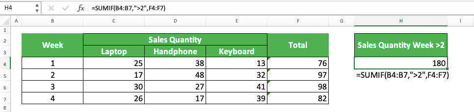
Here, we use the same data as the one we use to exemplify the SUMIF implementation previously. The difference is only in the shape of the table, which is now horizontal.
Because of that, we change the cell range inputs in the SUMIF to reflect that table shape too. We input the week and the sales quantity rows here so we can get our SUMIF result.
The criterion input is the same as if we write a vertical SUMIF. In this case, we write “>=6” for the criterion as we want to sum sales quantities for week 6 and beyond.
Not too big of a difference between horizontal and vertical SUMIF, right? Just remember to input row cell ranges in a horizontal SUMIF, while column cell ranges go into a vertical SUMIF.
Sum Numbers with a Cell/Font Color Criterion: XLTools
What if the criterion you have for your SUMIF is a cell/font color? Probably you have done a color code to your data table and you want to sum based on that.Unfortunately, Excel doesn’t have a built-in sum formula to do that. SUMIF also cannot sum based on a cell/font color criterion. However, if you have the XLTools Add-Ins installed in your excel, then you can do the sum easily!
To know how to do the sum using XLTools, follow these simple steps below.
For the steps illustration, let’s say we have a data table like below.
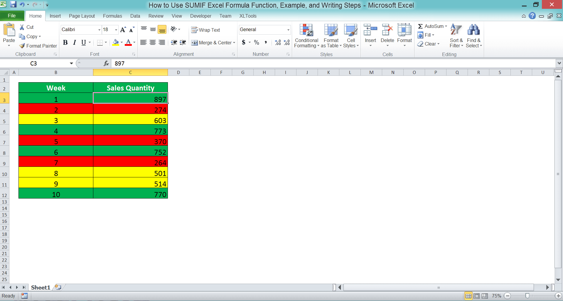
We want to sum the sales quantities according to the cell color criterion. How do we do it?
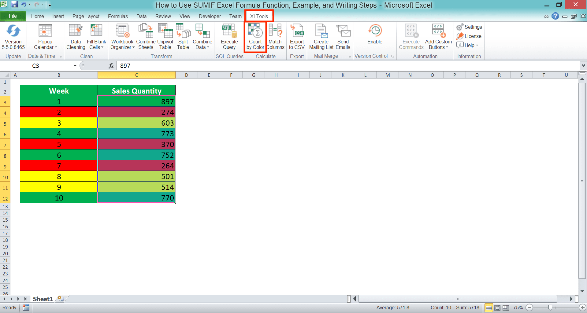
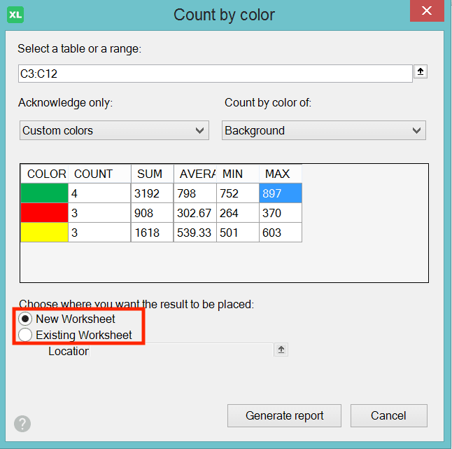
First, highlight the cell range containing the numbers we want to sum according to the cell color (in the example, that means the sales quantity column). Then, head to the XLTools tab and click the Count by Colors button there.
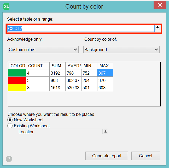
The button will open the XLTools’ Count by Colors dialog box. The cell range you highlight has been inputted to the text box there. The cell range in the text box is the one that will be processed by XLTools.
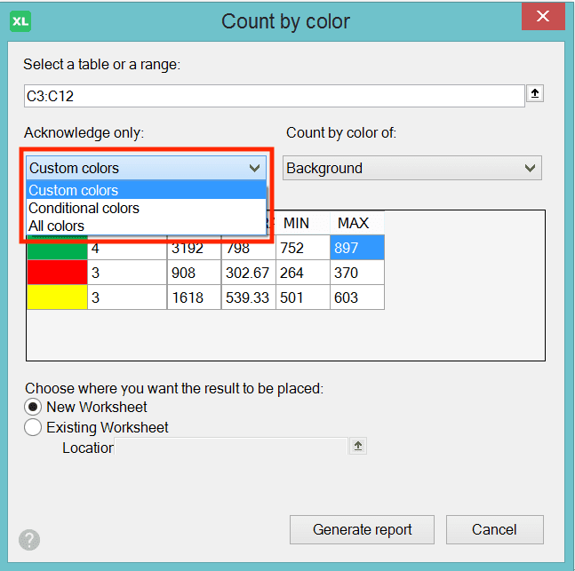
In the dropdown on the left below the text box, you can choose the kind of colors you want to process. The choices and their meanings are:
- Custom colors = the cell/font colors to process are the ones you color manually
- Conditional colors = the cell/font colors to process are the ones given by Conditional Formatting
- All colors = the cell/font colors to process are the ones you color manually and from the Conditional Formatting also
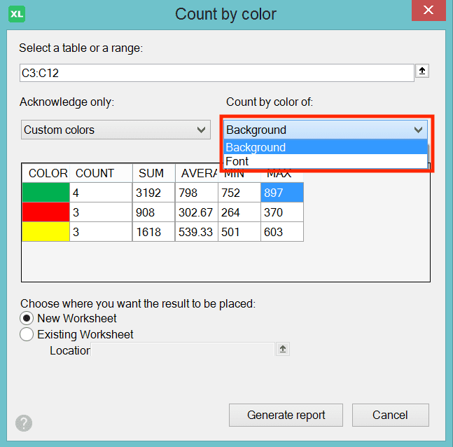
In the other dropdown, you can choose whether you want to process your numbers based on the cell or font color. Choose Background for the cell color and Font for the font color.
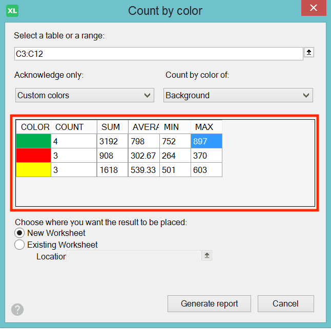
The screen below the two dropdowns shows the preview of the result you will get from the current settings. If you want to see the sum results, you can take a look at the SUM column there.
Below the preview screen is the location setting to determine where to put the result. Choose New Worksheet to make XLTools create a new worksheet and put your result there. Or choose the Existing Worksheet to put the result in the current worksheet.
If you choose Existing Worksheet, then XLTools will show a dialog box for you to input the location.
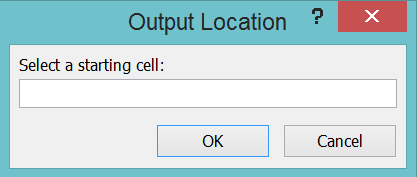
Just click on the most top-left cell where you want to put the result.
After all the settings are done, click the Generate Report button in the dialog box. Next, click Cancel.
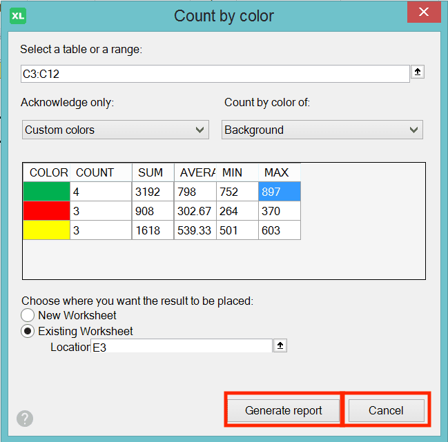
You have got the calculation results based on the color code you have in your numbers cell range!

If you only need the sum result, then delete all the other results you don’t need from there.
SUMIF with OR Criteria
What if we have multiple criteria and we want all the numbers which data entries fulfill at least one of them summed? For that, you can use this SUMIF with OR criteria method.This method actually just adds SUMIFs with the number of SUMIF you add depends on the number of your criteria. The general writing form of the SUMIF with OR criteria can be illustrated like this.
= SUMIF (data_range_1, criterion_1, [number_range_1]) + SUMIF (data_range_2, criterion_2, [number_range_2]) + …
Input each criterion you have on each SUMIF you write. The cell ranges you input depend on where you want to evaluate data and sum your numbers.
To make the concept clearer, see the example below.
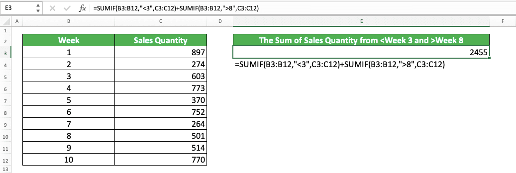
In the example, we want to sum the sales quantities from before week 3 and after week 8. Because there are two criteria and we need to sum both, we use multiple SUMIFs to help us.
We write one SUMIF for the before week 3 criterion (“<3”) and one for the after week 8 criterion (“>8”). Because both criteria cell ranges are the same (week and sales quantity columns), we input the same cell ranges for both SUMIFs.
Add the SUMIFs and we will get our SUMIF with OR criteria result!
SUMIF with AND Criteria: SUMIFS
If OR means the data has to fulfill at least one criterion, AND means the data has to fulfill all criteria. In AND, failing to meet one criterion means the number of those data entries won’t be summed.If this is what you need for your SUMIF result, then you should use the SUMIF sibling formula, SUMIFS.
You can check the full tutorial of SUMIFS here. However, in brief, you can write SUMIFS like this in excel.
= SUMIFS ( numbers_range, data_range_1, criterion_1, … )
In SUMIFS, you input the data range and its criterion in pairs. The criterion you input will only evaluate the data in the cell range before it.
You can input up to 127 pairs of criterion and data range. Before you input them, you need to input the cell range where the numbers you want to sum are.
As in SUMIF, you should make all the cell ranges you input in SUMIFS parallel and have the same size. SUMIFS will then sum the numbers from data entries in which adjacent cells fulfill all the criteria you have.
To better understand SUMIFS in excel, here is its implementation example.
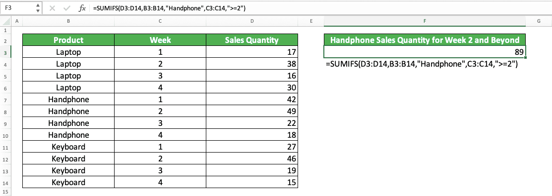
We want to sum the sales quantities of handphone in week 2 and beyond. How do we do it? We use SUMIFS, of course!
As explained before, first, we input the number cell range of the data entries. In the example, that means we input the sales quantity column. After that, we input the data ranges and their criterion pairing.
The criteria that we have are handphone product and week 2 and beyond. Therefore, we input the product column and the “Handphone” text in our SUMIFS. Next, we input the week column and the “>=2” criterion. You can input the product and week cell range and criterion in any order.
Do that SUMIFS writing and we will get the sum result that we want! This is the implementation of the SUMIF with AND criteria in excel.
SUMIF with the Criterion in a Separate Table: SUMIF VLOOKUP/SUMIF INDEX MATCH
Sometimes, we can have separate tables in excel and we need both data to input our SUMIF data and number ranges. We cannot just write SUMIF to sum the numbers we want there. If there is connector data between the tables, then we can use SUMIF with VLOOKUP/SUMIF with INDEX MATCH.The VLOOKUP or INDEX MATCH here functions as the formula that will connect both tables. From the connection, we can use SUMIF to sum numbers based on the criterion in a separate table.
Generally, here is the writing of SUMIF VLOOKUP for this purpose.
= SUMIF( data_range, VLOOKUP ( criterion, criterion_table_range, col_index_num, [ lookup_mode ] ), number_range )
And here is the writing if you prefer INDEX MATCH to VLOOKUP.
= SUMIF( data_range, INDEX ( connector_range, MATCH ( criterion, criterion_range, [ match_type ] ) , 1 ), number_range )
The INDEX MATCH writing there is for if the criterion table range data are divided into columns. If in rows, then you should swap the MATCH formula with the number 1 there.
In both writings, the VLOOKUP/INDEX MATCH there tries to find the connector data in the criterion cell range. VLOOKUP/INDEX MATCH will then give the connector data to SUMIF so it can become its criterion. From there, SUMIF will run its process and sum your numbers based on the criterion you have.
To make the understanding clearer, here is the implementation example.
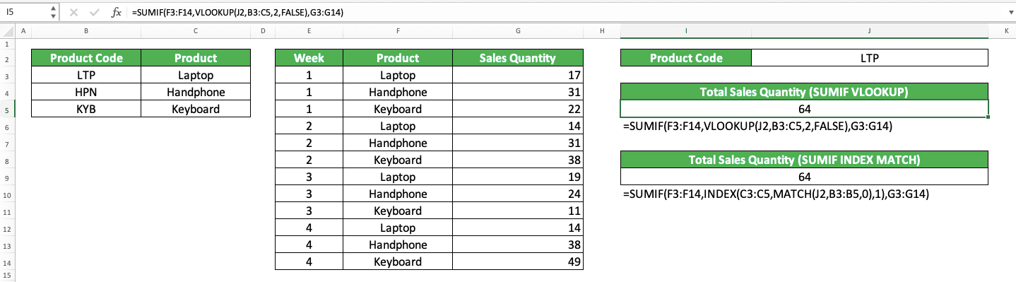
Here we have product code-product and product-sales quantity tables in our worksheet. We also have the product code we want to sum the sales quantity of. However, the product code data isn’t in the sales quantity table.
For this sum process, we can use the help of SUM VLOOKUP/SUM INDEX MATCH.
You can see the formula writings for both methods in the screenshot. The connector here is the product data because it has its place in both tables.
First, we find the product name from the product code we want to sum the sales quantity of. We do that in the product code-product table using VLOOKUP/INDEX MATCH.
After we find the product name, we use it as a criterion for our SUMIF. From there, we will get the sum of sales quantity for the product code we want!
It is a pretty complex operation. However, if you understand the usage principles of SUMIF and VLOOKUP/INDEX MATCH, you should be able to do it!
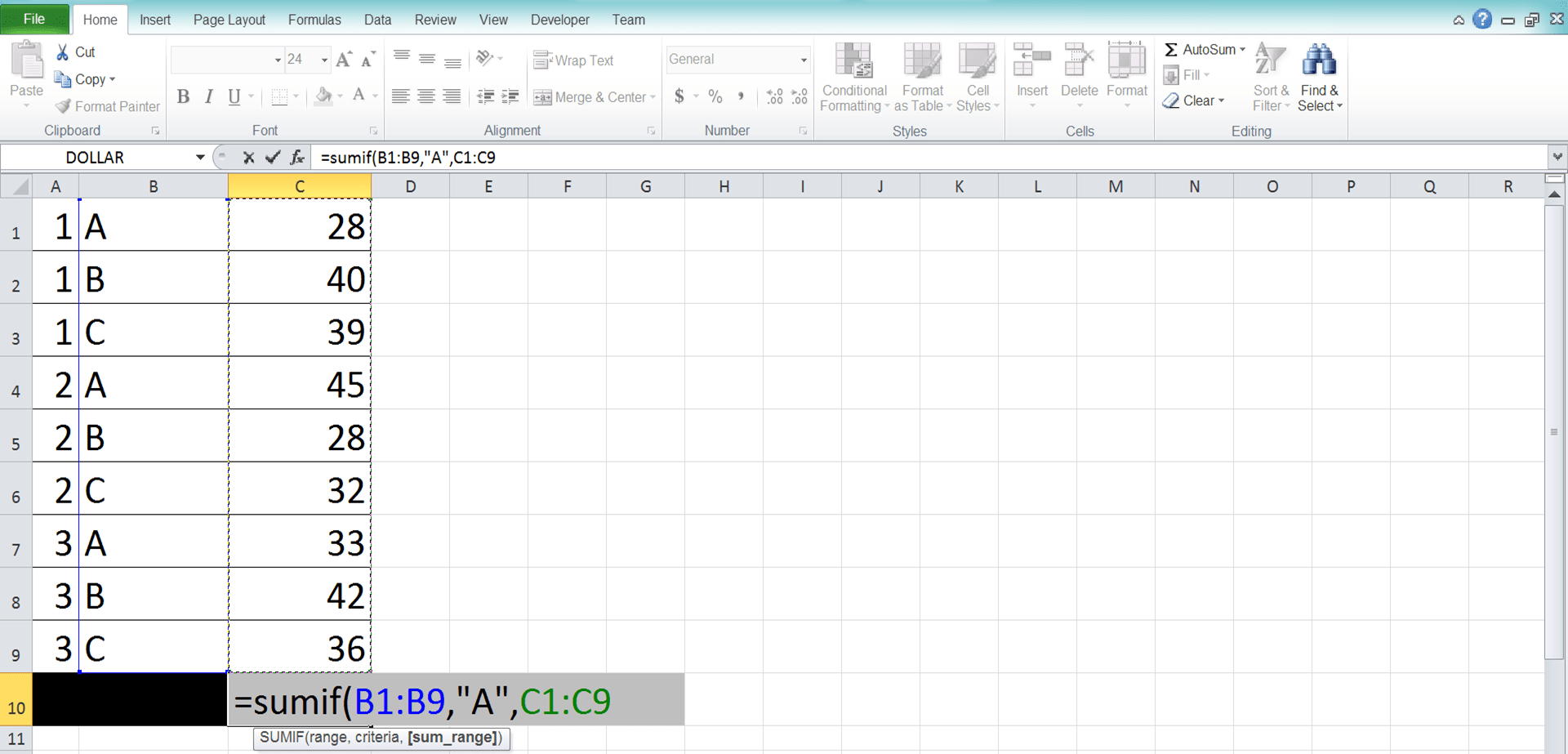
SUMIF for Multiple Number Columns
Now, what if we have one data cell range and multiple number cell ranges? We want to sum numbers from those number ranges if their data entries fulfill the criterion in the data range.How do we do that? Well, there are two ways to do it.
The first is to have a helper column and sum all the numbers in those number ranges per row. From there, we can input the helper column to our SUMIF to get our sum result.
The second is to sum all separate SUMIFs that we make per number range. That way, we can get the SUMIF result for multiple number columns.
Here is the implementation example for both methods.
The first method (helper column)
The second method (sum separate SUMIFs)

You can see how we use both methods to do SUMIF for multiple number columns above.
In the first screenshot, we sum our columns’ numbers first per row. From there, we use SUMIF to sum the numbers in the helper column from the data entries that meet the criterion.
In the second screenshot, we use multiple SUMIFs to sum each of the number columns. We sum all those SUMIF results to get the final sum result we want.
Both methods can give us the result we need in this case. It is up to you which one you might prefer in your excel work!
Exercise
After you have learned how to use the Excel SUMIF function, you can practice your understanding through the exercise below!Download the exercise file and answer the following questions. Download the answer key file if you have done the exercise file and sure about your answers!
Link to the exercise file:
Download here
Questions
- What is the total sales of product A?
- What is the total sales of products in region 1?
- What is the total sales of product B and C?
Link to the answer key file:
Download here
Additional Note
If you want, you can also use SUMIFS to sum numbers with just one criterion (as what the SUMIF formula is for).Related tutorials you should learn: