How to Use VLOOKUP Excel Formula

In this tutorial, you will learn how to use the VLOOKUP excel formula. VLOOKUP formula in excel is pretty important to learn because it can help to find your data in a cell range. Data lookup is one of the most important processes to understand if you want to analyze your data optimally.

To be honest, this VLOOKUP tutorial is quite long if you want to learn all its contents. This is because we discuss VLOOKUP from various perspectives based on the questions asked from excel users like you!

If you seriously want to master VLOOKUP, then learn this tutorial from the beginning until the end. However, if you don’t have the time, you can move to the tutorial part you need from the Table of Contents. Bookmark this tutorial if you want to learn the other parts later!

Disclaimer: This post may contain affiliate links from which we earn commission from qualifying purchases/actions at no additional cost for you. Learn more

Want to work faster and easier in Excel? Install and use Excel add-ins! Read this article to know the best Excel add-ins to use according to us!

VLOOKUP Usefulness

The VLOOKUP formula is useful to find data from a cell range vertically in excel.

Result

The result you get from VLOOKUP is the data you lookup for.

Excel Version in Which VLOOKUP Can Start to Be Used

You can use the VLOOKUP formula since excel 2003.

The Way to Write it and Its Inputs

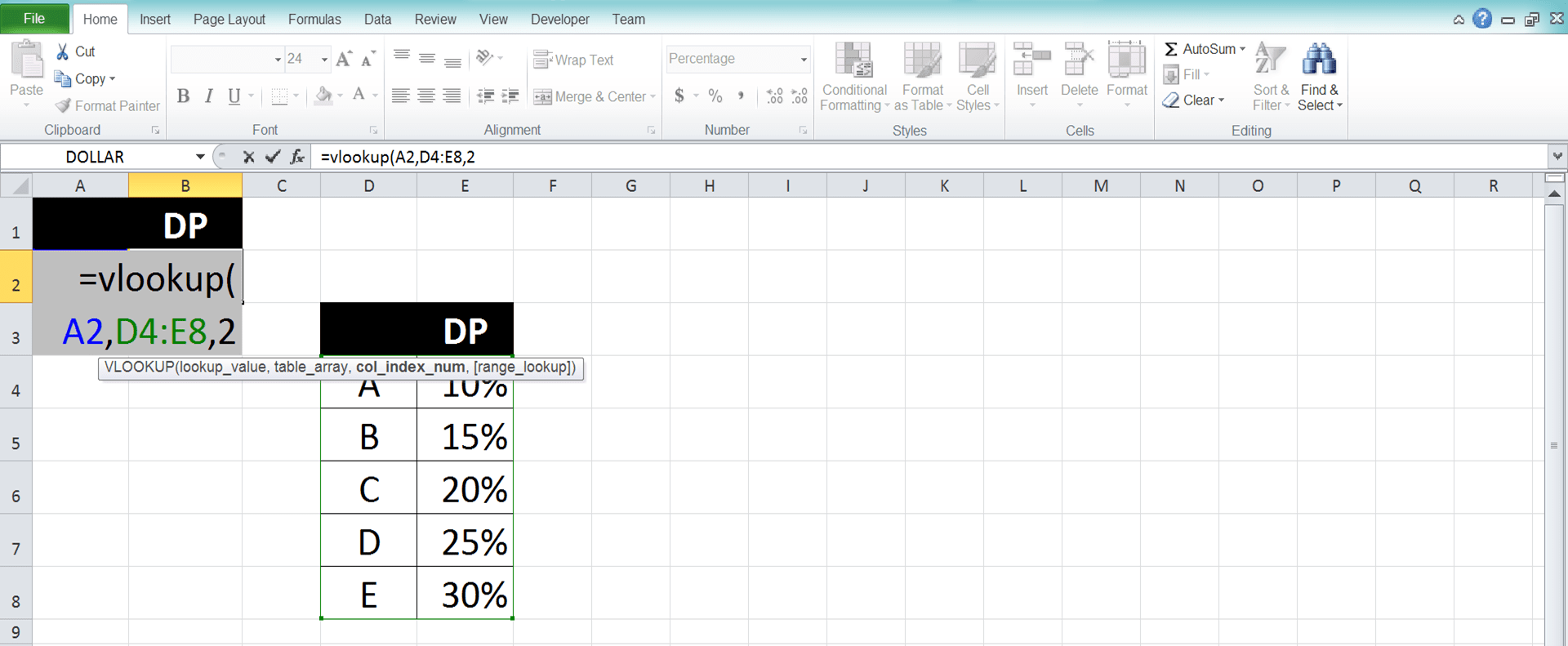
Generally, the way to write the VLOOKUP excel formula can be illustrated as follows:



The inputs you need to give in its writing can be explained as follows:

• lookup_value = the lookup reference value that needs to be found in the first column of your reference table cell range
• table_array = your reference table cell range
• col_index_num = the order position of the column on the reference table where the result of this formula will be taken (the order will be counted from the most left position)
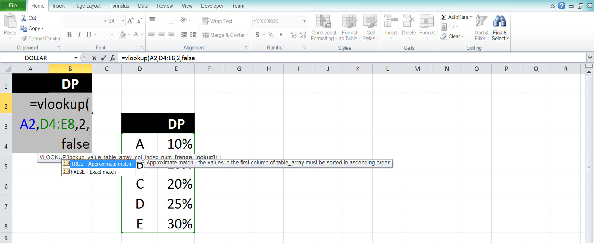
• [range_lookup] = optional. Determines whether lookup value will be searched for an exact or approximate match. TRUE for approximate and FALSE for exact

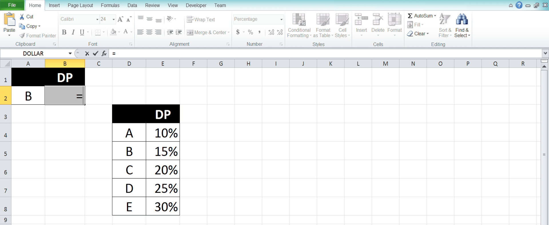
VLOOKUP Example 1: Biodata Search

The following will give and explain the first VLOOKUP example. It will show its usefulness, writing, and result.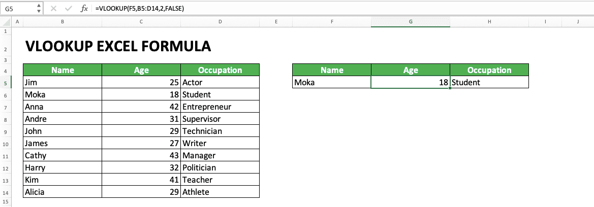



From the example, it is clear how VLOOKUP can be used to find data vertically. The way to use this formula itself is by giving it the inputs explained in the previous tutorial section correctly. Those inputs are the reference value, the cell range for the lookup process, the result column order, and the lookup nature.

The way this formula works is: it will look at your cell range’s first column and search your reference value there. When found, VLOOKUP will take its row position to your result column. If there is more than one match in the first column, it will take the row position of the top one.

Its last optional input, the lookup nature, is also important to understand. You can input TRUE/FALSE here with the default is TRUE if you don’t input anything. TRUE means if an exact match cannot be found, it will look for the smaller nearest value to the reference value. FALSE means if the exact match cannot be found, then it will produce an error.

It is important to remember that if the input is TRUE, you must sort the first column in ascending order. If not, then the result of your VLOOKUP excel formula can be wrong or even produce an error.

The practice of all this explanation can be seen in the VLOOKUP formula example above. In the example, we can see the reference value there is “Moka”. This formula will search “Moka” in the first column of the inputted cell range and pull data on the result column. In the example, we input 2 and 3, the order of “Age” and “Occupation” columns in the cell range.

Then, because the last input is FALSE for the VLOOKUP, the first column doesn’t have to be sorted. The combination of all those inputs gives the appropriate result for the data lookup need in the example.

VLOOKUP Example 2: Score Range and Its Letter Translation

The next example we can discuss to make our understanding clearer is the determination of score letters from their number ranges.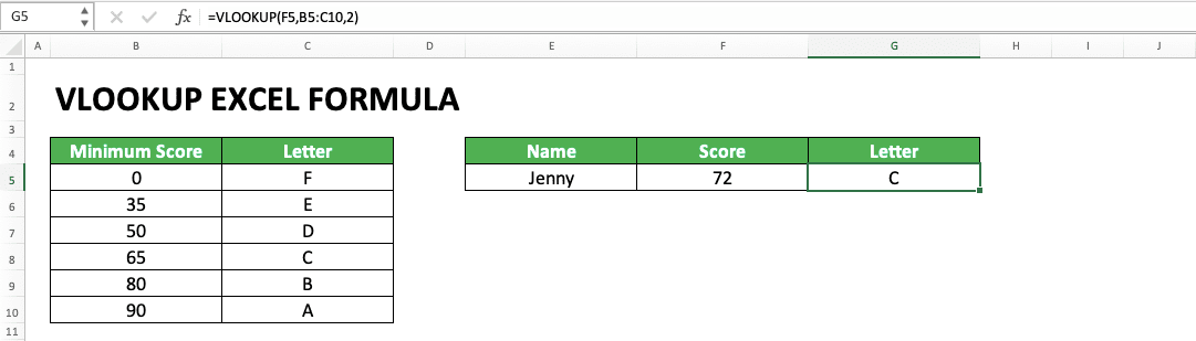



In the example, we can see how the VLOOKUP formula gives a result if the search nature is TRUE or approximate. When we want to change a score number to a letter, usually score ranges are the reference.



We can see from the example of how VLOOKUP converts a 72 based on the reference table on the left. As explained before, VLOOKUP automatically assumes its last input part as TRUE if we don’t give any input there. Because of that, the VLOOKUP formula writing in the example doesn’t need any input there (if we input TRUE there, then the formula result will be the same).

VLOOKUP with TRUE will prioritize the exact match first before looking for an approximate match. As seen in the reference table, there is no 72 there.

Because of that, VLOOKUP takes the row position of the smaller nearest score from 72, which is 65. Because the second column content (why the second column? It is based on the input of the result column order in the VLOOKUP) in line with 65 is C, then this score letter will be the VLOOKUP result.

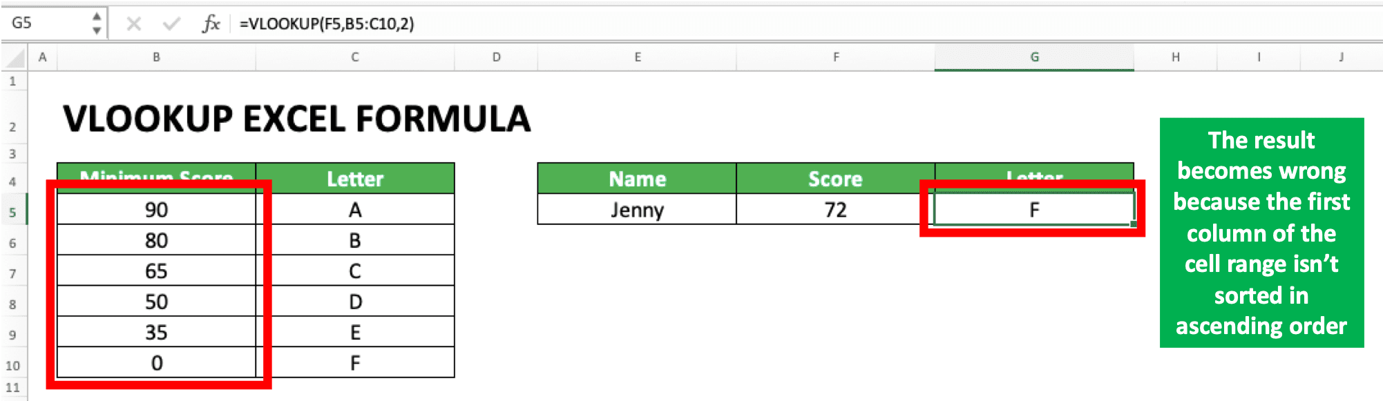
See also that the first column of the example’s reference table has been sorted in ascending order. This, once again, is important when we search for an approximate match using VLOOKUP. If it isn’t sorted, then most probably the VLOOKUP result will be wrong or an error. You can see the example of this in practice in the following screenshot.

VLOOKUP Example 3: Manual Number-to-Text Formula

The next example is a VLOOKUP application you can use to change your number into its text version.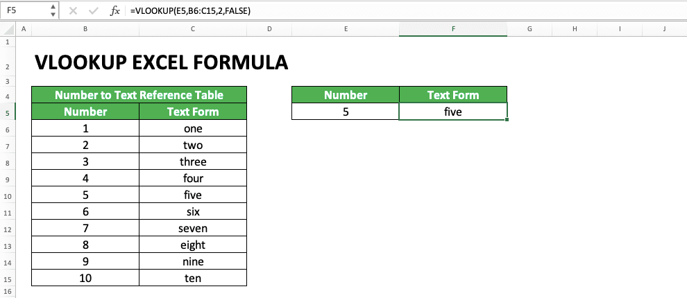



In the example, we can see how VLOOKUP can be a number-to-text formula in excel. As long as there is an appropriate reference table, it can change a number into its text form. Make sure its search nature input is FALSE so it won’t pull the wrong text from the reference table.

If you want to convert decimal numbers or numbers above ten, you need to have more contents in the reference table. If you want a more practical way of getting the text version of a number, you can create a VBA formula. The tutorial on how to create it can be learned here.

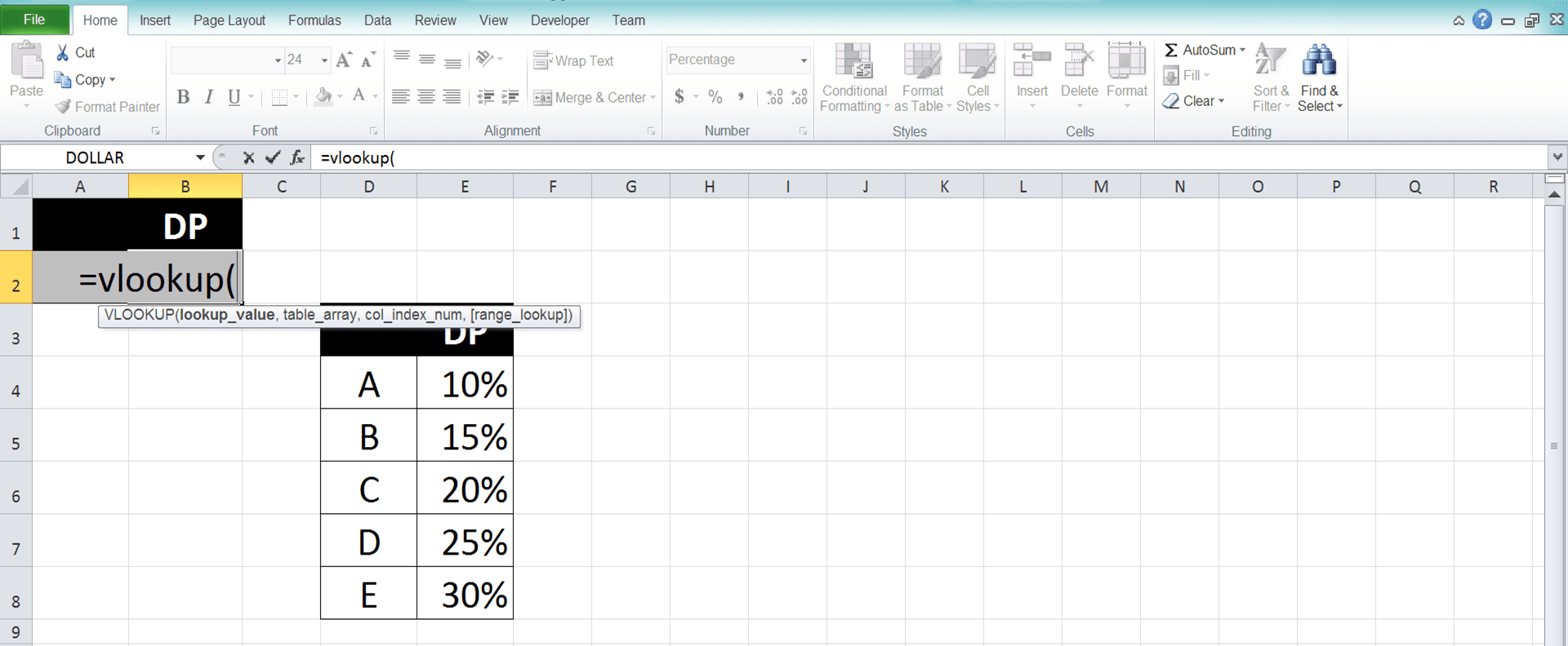
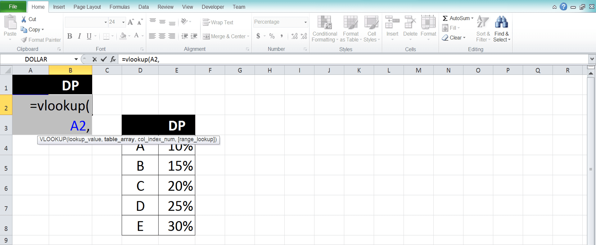
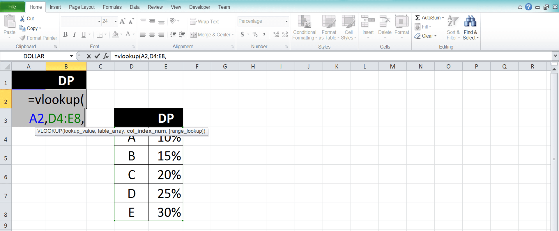
Writing Steps

The VLOOKUP writing explained in step-by-step will be given in the following part of the tutorial. The way to use the VLOOKUP formula itself is quite complicated to understand if you haven’t learned it previously. Because of that, the VLOOKUP writing example will be given in the form of screenshots for each step. Hopefully, that makes the explanation much easier to understand!

1. Type an equal sign ( = ) in the cell where you want to put the result
   
   
   
   
2. Type VLOOKUP (can be with large and small letters) and an open bracket sign after =
   
   
   
   
3. Input the lookup reference value or the cell coordinate where the value is. This value will be searched later in the reference table. Then, type a comma sign ( , )
   
   
   
   
4. Drag cursor on the cell range where your reference table is then type a comma sign. Later, the lookup reference value inputted earlier will be searched in the first column of this reference table
   
   
   
   
5. Input the nth order of the column where your lookup result should be found in your reference table. The result will be gotten from where the row in which your lookup reference value is found combined with this column. If there is more than one matches found for the lookup value, it will get the one on the top
   
   
   
   
6. Optional: To determine whether the lookup value must be found exactly or just approximately, do this. Input a comma sign and type TRUE/FALSE (can be with large and small letters).
   
   TRUE for approximate and FALSE for exact. The definition of approximate is if there is no exact similar value, then it will do this. It will make the smaller nearest value from the lookup value in the reference table’s first column as a reference.
   
   As an important note, you must sort the value in the first column in ascending order so the TRUE functions correctly. If there is no input from you in this part, then the input will be considered as TRUE
   
   
   
   
7. Type a close bracket sign
   
   
   
   
8. Press Enter
9. The process is done!
   
   
   
   

Explanation About TRUE/FASE in the VLOOKUP Function (Lookup Nature/Mode)

You should pay attention to the TRUE or FALSE input in the VLOOKUP because it is crucial to determine your result. As explained before, you should input TRUE if VLOOKUP can look for an approximate of your lookup reference value. Input FALSE if it must be an exact match.

If you input a TRUE lookup mode, then VLOOKUP can take a smaller nearest value from your lookup reference value. If FALSE, then if VLOOKUP doesn’t find an exact match with your lookup reference value, it will return an error.



If you don’t input anything in this part, then the VLOOKUP will consider your input as TRUE. It can have an approximate match.

Use the TRUE/FALSE input as you need it. However, you must remember if TRUE, the first column where you look for a match must be sorted in ascending order. If not, then the VLOOKUP result can be wrong or an error.

The error because the first column hasn’t been sorted is also one reason why VLOOKUP often not working in someone’s excel.

Factors That Can Make VLOOKUP Produces an Error

VLOOKUP sometimes doesn’t produce the result we want or even an error. Factors of why that happens should be paid attention to so we don’t do mistakes in using the VLOOKUP.

From many reasons that can be factors of a VLOOKUP error, here are 3 that most probably cause it:

• Using TRUE as the lookup mode/nature input but the data in the first column isn’t sorted in ascending order
• The lookup reference value isn’t found in the first column of the reference table cell range
• Wrong inputs for the reference table cell range and/or the result column order

Pay attention to your VLOOKUP usage so it doesn’t apply those error factors.

Anticipate an Error from VLOOKUP: IFERROR VLOOKUP

Probably we have tried hard to avoid an error in our VLOOKUP writing. However, sometimes an error can still be produced from the formula. This can make further data processing from the VLOOKUP result error too.

What can we do to anticipate the error and make it not disturb our data processing? The answer is to combine our VLOOKUP writing with an IFERROR.

Generally, the writing of the IFERROR and VLOOKUP formulas combination can be illustrated as follows:



The input explanation for the VLOOKUP writing above is the same as explained in the previous part. For the IFERROR, value_if_error is the value we want to produce if your VLOOKUP produces an error.

The example of the IFERROR VLOOKUP use in excel is as follows:



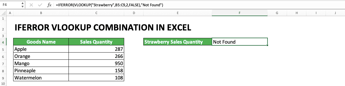
In the example, we can see how the IFERROR VLOOKUP combination is written. Because of the IFERROR, the VLOOKUP error result is changed to “Not Found” text there. If there is no IFERROR, then the VLOOKUP will produce an #N/A error.



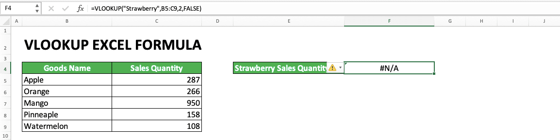
The alternative value in the IFERROR input is usually words like “Not Found” or empty data (“”). But, of course, it is up to you what kind of alternative value you want to use in the formula combination.

VLOOKUP With Wildcard Characters

In the lookup reference value of VLOOKUP, we can also use wildcard characters. For those who don’t know about them, they are the characters that can be replaced with any other characters.

In excel, there are two kinds of wildcard characters you can use:

• Star sign (*): can be replaced by any character in any amount
• Question mark (?): can be replaced by any character with the amount of one

If they are used in VLOOKUP, The wildcard characters are usually put in the lookup reference value input part. Their implementation examples in the VLOOKUP can be seen in the screenshots below:





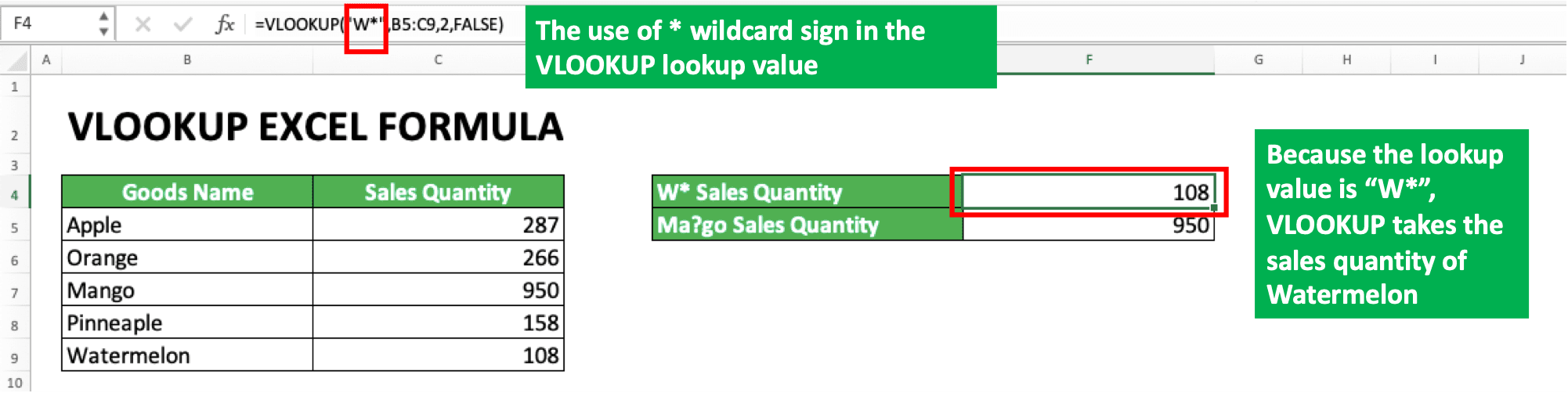
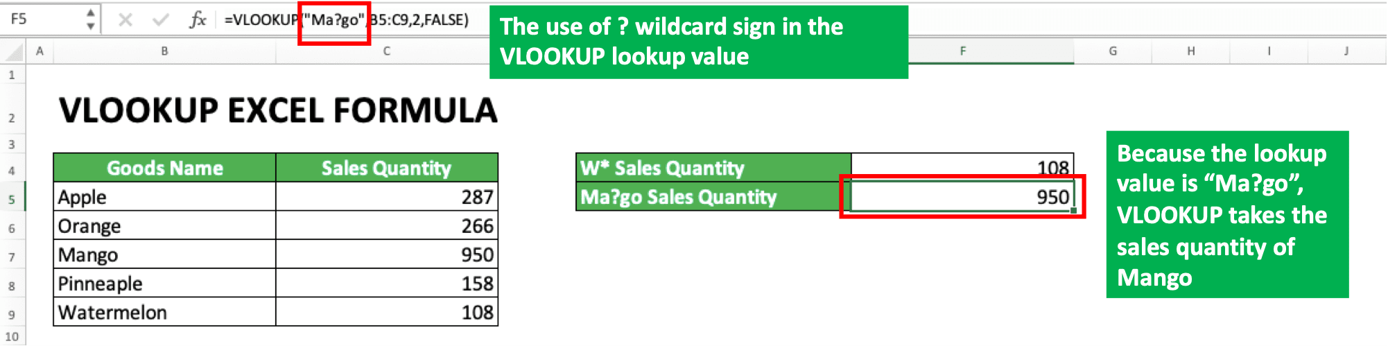
In the two examples, we can see the impact of * and ? symbols in the VLOOKUP lookup reference value. The * in the “W*” makes VLOOKUP looks for data with the “W” prefix. Meanwhile, the ? symbol in the “Ma?go” makes VLOOKUP looks for data with the “Ma” prefix and “go” suffix.



In the example, we can also see the * sign can be replaced with any character in any amount (“W*” can mean “Watermelon”, “Water Lemon”, or other words as long as it has a W prefix). The ? symbol, on the other hand, only represents one free character (“Ma?go” can mean “Mango” or “Maxgo” but cannot mean “Mannnnnnnngo” or “Maxijago”).

The use of * and ? wildcard symbols themselves can be in whichever part of your lookup reference value in VLOOKUP. However, if you want to use the * and ? symbol in your lookup reference value, use ~ sign in front of them (example: The lookup reference value of “Hard~?” will make VLOOKUP look for “Hard?” text not “Hardy” or “Hards”).

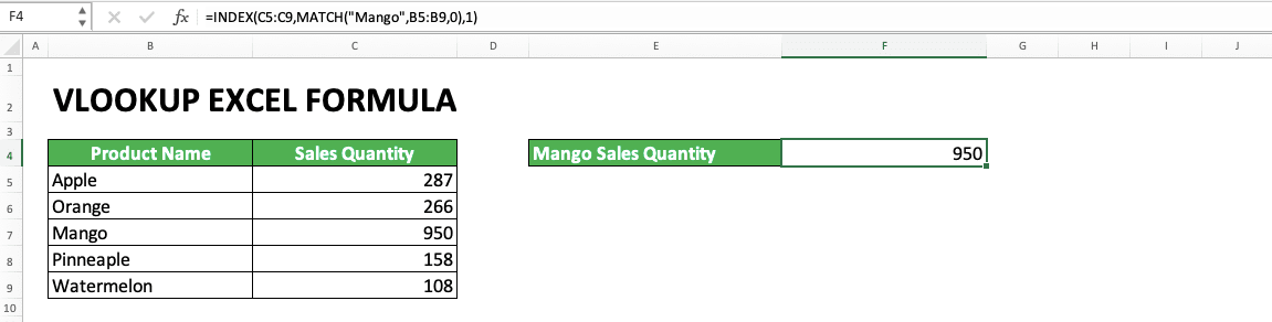
VLOOKUP to the Left

The VLOOKUP data lookup process always looks to the right. It looks for your lookup reference value on the most left column of the cell range. After that, it finds its result on the right of that column.

How about if the lookup reference value is on the right of the column where we want to get the result? The solution is by not using VLOOKUP to look for your data. You should use INDEX MATCH instead.

INDEX MATCH is a combination of the INDEX and MATCH formulas in excel. It can make your data lookup process more flexible. If you want to learn this formula deeper, follow its tutorial from Compute Expert here.

The following is the INDEX MATCH usage example to find data with the lookup process to the left.



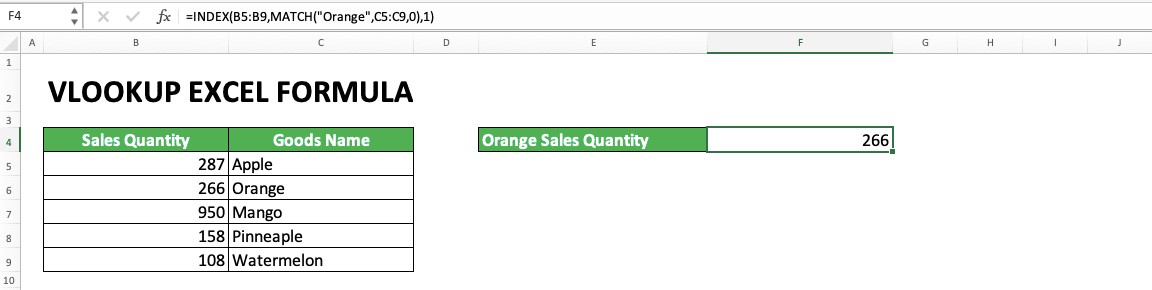
As you can see in the example, INDEX MATCH can be utilized to find data to the left. This is because its cell range and lookup reference value nature are more flexible. The INDEX and MATCH cell ranges can be put anywhere with the lookup reference value is inputted in the MATCH formula.

INDEX MATCH is different from the VLOOKUP limitation which requires one cell range for the lookup reference value and its result. This causes the VLOOKUP lookup process to just can be done to the right.

So, if you seriously need a lookup process to the left, then use INDEX MATCH to get your data.

VLOOKUP With a Reference Table on a Different Sheet

A question often asked about VLOOKUP is: How to write a VLOOKUP if the reference table is on a different sheet?

The writing is similar to the VLOOKUP which has the reference table in the same sheet. It is just when inputting its cell range, you must click the sheet where the reference table is first.

Then, drag your cell cursor in the reference table cell range before you go back to your VLOOKUP sheet and cell. From there, you just need to continue your VLOOKUP writing as usual.

To make it clearer, probably you should see the screenshot below. In the screenshot, we can see the reference table is in a sheet named “Sheet1”.



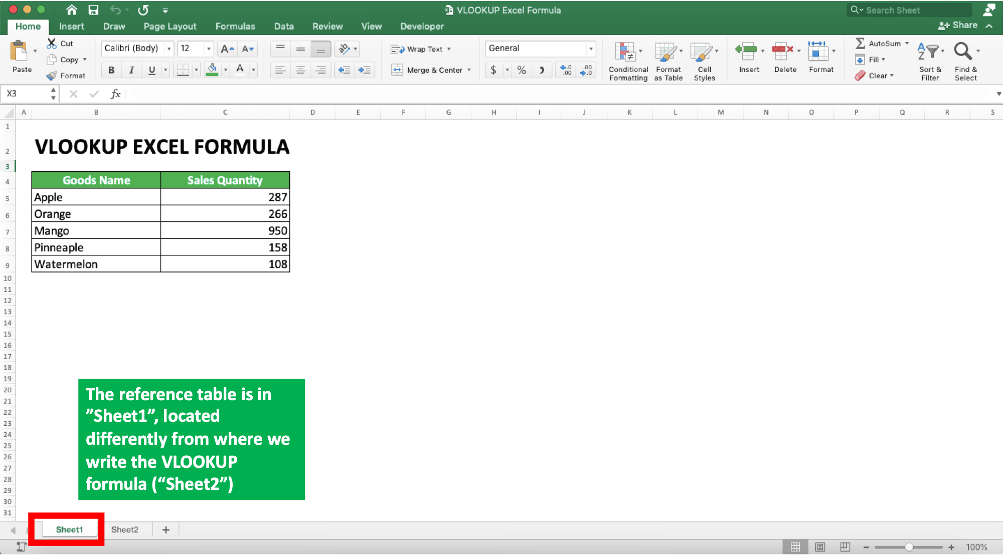
We want to write the VLOOKUP in the sheet named “Sheet2” which is different from the reference table sheet. How to write the VLOOKUP for this? Here is an example of writing with that condition.



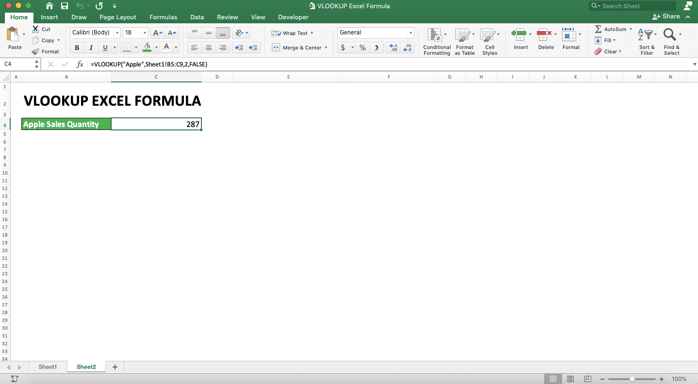
As you can see in the formula bar above, in the cell range input, the writing is Sheet1!B5:C9. A writing like that is automatically inputted if you move to “Sheet1” and drag your cursor on cell B5 to C9.

Or if you want to type the cell range input directly, don’t forget to write it in that format (Sheet_Name!Cell_Range). That writing format for a reference table in a different sheet is important so your VLOOKUP can function as intended.

After inputting the cell range where VLOOKUP will look for the data, you just need to give other inputs normally (like when the reference table is on the same sheet as your VLOOKUP).

VLOOKUP With a Reference Table on a Different File

What if the reference table you want to use is on a different file? The answer is you must input your reference table’s cell range by considering its excel file name and its sheet name.

Check the following example. Let’s say the reference table you want to use in your VLOOKUP is in the file named “Book2.xlsx” (xlsx is the extension used by this excel file). The file is different from the place where you write your VLOOKUP.



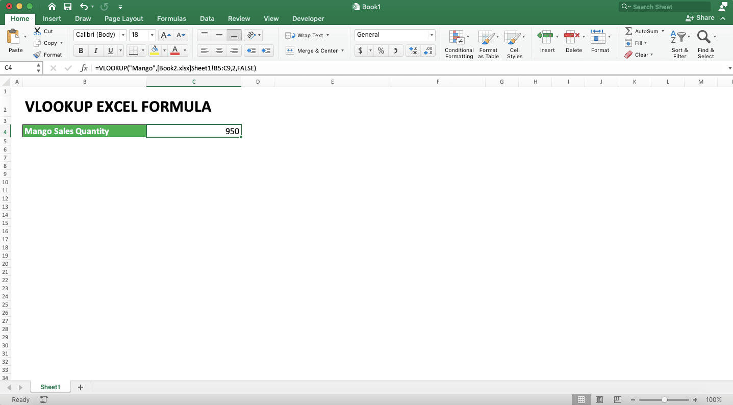
How to refer to the reference table? Write its excel file name and its sheet name before its cell range in your VLOOKUP input!

The writing format is like this if your reference table file is also opened currently: [Workbook_Name]Sheet_Name!Cell_Range. As an example, look at the screenshot below for the VLOOKUP writing in a different file with the “Book2.xlsx”.



After opening the excel files (the file where your VLOOKUP is and where the reference table is), go to the reference table file while putting the reference table input in your VLOOKUP.

Then, drag your cursor on the cell range where the table data is. Next, type a comma and go to your VLOOKUP file again. After that, you just need to give the rest of the VLOOKUP inputs as usual.



If you want to type the cell range directly, then type in something like [Book2.xlsx]Sheet1!B5:C9. Do that when your reference table file is opened. If it is currently closed, then you must type in the file’s pathname too (e.g. ‘C:\Documents\[Book2.xlsx]Sheet1’!B5:C9 (Windows) or ‘/Users/Documents/[Book2.xlsx]Sheet1’!B5:C9 (Mac)).

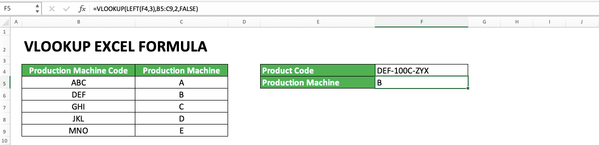
VLOOKUP With the Lookup Reference Value That is a Part of a Cell Content

If the data you look for is just a part of your lookup reference value, you can use the wildcard characters. However, what if you just need a part of cell content for your lookup reference value? For this, you need to combine your VLOOKUP writing with the LEFT, MID, or RIGHT formulas.

The explanation of these formulas can be learned in the links given. Those three formulas can help us finding some characters we have in cell content data.

Which of those three combined with the VLOOKUP depends on the cell content part position used as the lookup reference value. Use LEFT if the part is on the left, MID if middle, and RIGHT if it is on the right. They can be used to separate the cell part from the whole cell content before it is used in your VLOOKUP.

The usage example of each of the three formulas, when combined with VLOOKUP, can be seen below.

VLOOKUP-LEFT:



VLOOKUP-MID:



VLOOKUP-RIGHT:



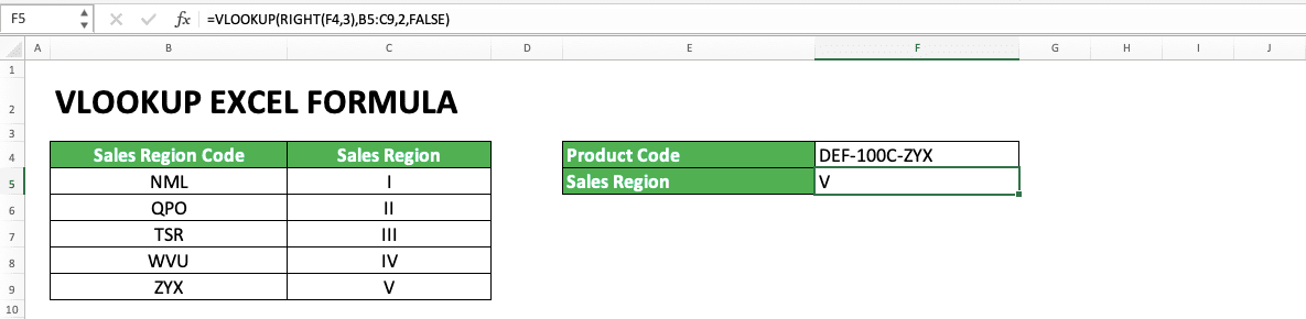
Sometimes, a product code in a company has parts that can be translated into information. The LEFT, MID, or RIGHT combination with VLOOKUP can help us translate the information as seen in the example.

In the combination writing, we put LEFT/MID/RIGHT in the lookup reference value input part of our VLOOKUP. Decide how many characters we want to take from the left/middle/right position according to the formula used. LEFT/MID/RIGHT will function for the VLOOKUP with the lookup reference value that is a part of cell content.

Each of the three formulas has its usefulness depending on the data part position you want to take. Use the formula you need in your VLOOKUP!

VLOOKUP With the Nth Match (Not the First Match)

In its process, VLOOKUP will automatically take the first match with our lookup reference value in the cell range’s first column. What if we need the second or third match? For this, you better make a helper column on the left of this first column to help you.

To make the understanding clearer, see the example below.



We make a “Helper” column that contains data from the column where we want to look for our lookup reference value. We combine the data with its order there.

Later, our lookup reference value is also inputted with the order. The VLOOKUP cell range will also include the “Helper” column. The “Helper” column becomes the first column of the cell range in which the lookup reference value will be searched.

The example of these lookup reference value and cell range inputs can be seen in the example’s formula bar. As you can see, they are modified when we want to find the nth match of our VLOOKUP lookup reference value.

To fill the “Helper” column with the first column data order, we can create a formula to do it fast. An example of this formula can be seen below.



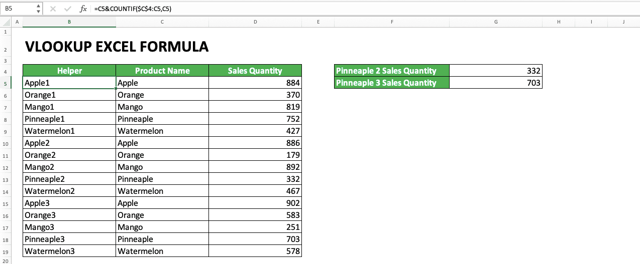
We use the help of & symbol and COUNTIF to help us write the formula. The & symbol is used to join the first column data with its order. Meanwhile, COUNTIF is used to create the order (if you haven’t understood how to use COUNTIF, you can learn it in this tutorial)

How to write the COUNTIF so it can produce this order? This can be seen in the screenshot’s formula bar above.

We input the COUNTIF’s cell range from the first column’s header cell until the parallel cell with our “Helper” column cell. We make the header cell coordinate in the cell range absolute so it doesn’t move when we copy our COUNTIF down. The absolute nature will make the COUNTIF counting scope always be from the header cell until the COUNTIF’s parallel cell (however down the COUNTIF is copied).

The COUNTIF criterion here is the parallel first column data for which we want to make the order. Because the cell range is inputted as explained before, this makes our COUNTIF produces the data order.

If the header cell until the parallel cell already has 2 similar data, COUNTIF will produce 2. If three, then COUNTIF will produce 3. This makes COUNTIF an appropriate formula to produce the data order number.

We will fill the “Helper” column with the first column data joined with the order number. In the VLOOKUP writing, we then use the “Helper” column to find our nth lookup reference value. We can determine the n as we prefer.

VLOOKUP With 2 or More Search Criteria/Reference Values

What if we want to use VLOOKUP but there are two or more columns contain the value we want to lookup? Almost similar to the nth match VLOOKUP, we need to create a “Helper” column and join those columns data there. We can see an example of this below.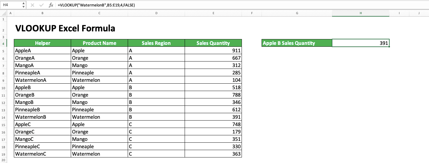



The key to use VLOOKUP with 2 or more more search criteria/reference values is combining all of them into one writing. This is needed for the VLOOKUP cell range first column and the lookup reference value.

In the example, we need to find the apple sales quantity in region B. Because there are two criteria there, apple and region B, we need to combine them in the lookup reference value input. As seen in the formula bar, we make the VLOOKUP lookup reference value to “AppleB” to accommodate the need.

In the VLOOKUP cell range, we add the “Helper” column so it becomes the first/most left column. The “Helper” column cell contents are the combination between the “Product Name” and “Sales Region” columns data. After all, these two columns’ data are the ones we want to make as our search criteria.



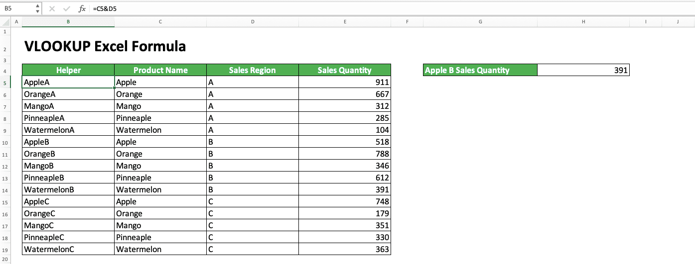
How to combine the data from the two columns? You can see how in the screenshot’s formula bar above.

Use the & symbol between the parallel cell coordinates of those two columns. Then, you just need to copy the data combination formula with the & symbol down to get all the combinations you need.

After that, you just input the lookup reference value and the “Helper” column in your VLOOKUP formula. You will get the data lookup result with 2 criteria/lookup values!

For more than 2 criteria/lookup values, you just need to combine more in your lookup reference value and “Helper” column. Make sure the “Helper” column is always on the most left of your VLOOKUP cell range input. This is so your data lookup process can run as intended.

VLOOKUP With a Dynamic Reference Table

When using a VLOOKUP, you probably want to determine your reference table cell range based on a certain cell value. A value means using reference table 1, B value means using reference table 2, and so on.



How to do it? The combination of IF and VLOOKUP is the answer.



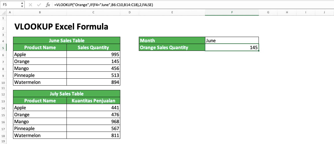
In the screenshot above, we can see the data lookup result if the month cell value is June. If the value is July, the result will refer to the July sales table as can be seen in the following screenshot.



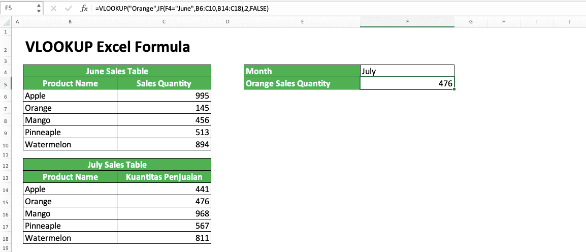
How to write a VLOOKUP formula that can change its reference table based on a cell value? The IF formula is essential here with its usage in the VLOOKUP cell range input.

Input the IF logic condition by making it refer to the cell we want. Then, if TRUE, input the reference table cell range we want for that. If FALSE, input another reference table cell range.

For more than 2 reference tables, you just need to input nested IFs in the VLOOKUP cell range input. Input as many IFs as you need according to the reference table cell ranges you need for the VLOOKUP.

VLOOKUP With a Dynamic Result Column

Beside a dynamic reference table, you probably also want to determine the result column order based on a particular cell content. For that, you need the combination of IF and VLOOKUP too. However, for the dynamic result column, you need to put your IF in the result column order input of your VLOOKUP.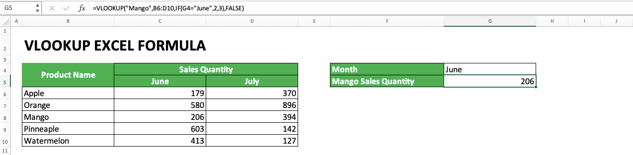



The example above shows how the combination of IF and VLOOKUP is done to make a dynamic result column. If the month cell value is replaced with July, then the VLOOKUP will get its result in the July column.



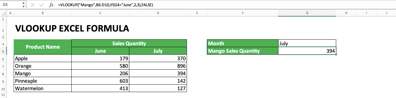
This VLOOKUP behavior can be gotten with a correct IF writing in the result column order input. Put the cell value you want as the determinant in the IF logic condition. Then, input the result column order if the cell value matches the logic condition you make. Input the result column order also if it doesn’t match.

If there are more than two columns you want for the VLOOKUP, use the nested IFs implementation in your VLOOKUP. Input as many IFs as you need according to the choices of result column orders.

Lookup Data Horizontally: HLOOKUP

As explained in the previous part, VLOOKUP is used if you want to lookup data vertically. It bases its lookup process on a cell range’s columns. Besides that, it also gets its result by finding the data row that fits its lookup reference value.

What if we want to lookup data horizontally, the opposite of the VLOOKUP process? One of the ways to do it is by using the VLOOKUP sibling formula, HLOOKUP.

In line with the first letter of the formula name, HLOOKUP will look for data in your cell range horizontally. It will do its search based on rows. Moreover, it will get its result by finding the column of the data that matches its lookup reference value.

Generally, the HLOOKUP formula writing can be explained as follows:



At a glance, the HLOOKUP input is almost the same as VLOOKUP. It is just HLOOKUP needs a result row order, not a result column order, in its input. Besides that, it also looks for its lookup reference value in the first row (not the first column like VLOOKUP) in its cell range.

The TRUE/FALSE search nature of HLOOKUP itself is the same as VLOOKUP. Don’t forget to sort your first row in ascending order when using a TRUE input.

Here is an example of HLOOKUP usage in excel.



From there, we can see how the HLOOKUP writing is done and how it works. In the example, HLOOKUP looks for a smaller nearest number to 82 in the first row of the cell range (because the search nature input is TRUE and there is no 82 in the first row). When found (60), it will look at its column position before taking the data in its result row to get a result.

If you want to learn more about HLOOKUP, please go to its specific tutorial here.

VLOOKUP Alternative: INDEX MATCH

VLOOKUP can be very rigid in its implementation. It is only limited to vertical data search and it can only process its search to the right. Besides that, its reference lookup value can only be searched in the first column of its cell range input.

Want a more flexible formula for all of those aspects? Use the INDEX MATCH combination.

Separately, INDEX is a formula that can produce data based on its cell range, column position, and row position inputs. On the other hand, MATCH is a formula that can give you position of data in a row/column.

Together, their combination can become a great data lookup formula. In our opinion, the INDEX MATCH is even better than VLOOKUP if you have understood how to use it.

An example of INDEX MATCH usage can be seen below.



From the example, you can see the writing and result of INDEX MATCH in Excel. Generally, you need to input MATCH in INDEX in the input part where you need to look for your data. Input MATCH in the INDEX row position input if the data you look for needs to be searched in a row. Oppositely, input MATCH in the INDEX column position input if your data needs to be searched in a column.

Want to learn more about INDEX MATCH? Learn it in this Compute Expert tutorial.

Exercise

After you have learned how to use the VLOOKUP excel formula correctly, now is the time to do an exercise. It is done so you can deepen your understanding of how to use VLOOKUP.

Download the exercise file and answer the questions. Download the answer key file if you have answered all the questions and want to check your answers. Or probably when you are confused about how to use VLOOKUP to answer all the questions!

Link to the exercise file:
Download here

Questions

Answer each question in the appropriate gray-colored cells by using a correct VLOOKUP formula!

1. What is the sales value of region E based on the reference table?
2. What is the sales quantity of region M based on the reference table?
3. How many salespeople are there in the sales region with the sales quantity smaller and the closest to 2000?

Link to the answer key file:
Download here

Additional Note

Maybe you have realized that you don’t need to include your table header in your VLOOKUP reference table cell range input. The most important thing is the place where you put the data needed for the lookup process has been inputted.



Related tutorials you should learn: