How to Divide Numbers in Excel


In this tutorial, you will learn various ways to divide numbers in excel.
When processing number data, one of the most basic calculations you can do to them is division. If you often use excel to process your numbers, then it is important to understand number dividing methods in this software.
There are two division-related formulas you can use in excel, although they don’t give you normal division results (as you will see later in this tutorial). There are also some methods you better understand to enable you divide numbers in excel optimally. Those methods involve some specific writing ways you should implement in your cells.
Want to learn those formulas and those methods? Then read all the parts of this tutorial completely!
Disclaimer: This post may contain affiliate links from which we earn commission from qualifying purchases/actions at no additional cost for you. Learn more
Want to work faster and easier in Excel? Install and use Excel add-ins! Read this article to know the best Excel add-ins to use according to us!
Table of Contents:
- How to divide numbers in excel normally using a manual formula writing
- How to divide cells in excel
- How to divide numbers without remainder in excel: the QUOTIENT formula
- How to get the remainder of a division calculation in excel: the MOD formula
- How to divide columns in excel
- How to divide a column by a number (constant) in excel
- How to divide a number with a percentage in excel
- How to handle a #DIV/0 error
- Exercise
- Additional Note
How to Divide Numbers in Excel Normally Using a Manual Formula Writing
The most common way to divide numbers in excel is by using the slash symbol ( / ) on our keyboard. Using the symbol, we write a division formula manually in our cell to get the calculation result we want.Generally, here is the way to write a division formula using the slash symbol in excel.
= number_to_divide / divider_number
Pretty simple, isn’t it? It is just like writing a standard division formula, in excel.
You just need to input the number you want to divide, a slash symbol, and the divider number too. Don’t forget to type an equal symbol ( = ) so excel recognizes the formula and runs the division calculation automatically.
Here is an example of the manual division formula writing in excel, where we divide 10 with 2.
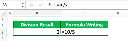
You can see how to write the division formula for the 10 and 2 calculation. Just write “=10/2” in your cell, following the writing pattern explained earlier, and you will get your result immediately!
How to Divide Cells in Excel
That is how it is done if we type our numbers directly into our division formula. But, what if we have put our numbers in excel cells and we want to divide them directly from there?Thankfully, Excel provides a way to refer to our cells directly to get their values for our formula writing. We just need to input the cells’ coordinates when we should input our numbers in the formula.
Here is the general writing form to divide cells with a number in them in excel.
= cell_coordinate_number_1 / cell_coordinate_number_2
Almost similar to the writing form if we type the numbers directly, right? The difference here is we input cell coordinates instead of direct numbers. A cell coordinate reference in an excel formula is inputted with the cell’s column letter and row number.
For example, we may write A1 as a cell reference. A is the cell’s column letter and 1 is the cell’s row number. Both make the cell position that we refer to becomes clear to us.
To make you understand the concept easier, here is an example of dividing cells in excel. We also divide 10 with 2 here as in the previous part of the tutorial.
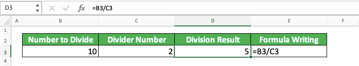
As the numbers we want to divide are already in their cells, we just refer to them in our division formula. The 10 is in the B3 cell and the 2 is in the C3 cell. Thus, we write our division formula as =B3/C3. We can input the cells by clicking on them or by typing their cell coordinates directly.
Refer to the number cells correctly and don’t forget to type the equal & slash symbols. Doing that, you will immediately get your division calculation result!
How to Divide Numbers Without Remainder in Excel: The QUOTIENT Formula
When we divide numbers, the result is often not a whole number. We often get decimals too as a remainder of the division calculation that we do.What if we want to exclude the remainder and just want to get the whole number result from our division? Is there a way to do that in excel?
Well, there is an excel formula you can use to get that kind of result. It is the QUOTIENT formula and the way to use the formula is quite easy!
Here is the general writing form of QUOTIENT in excel.
= QUOTIENT( number_to_divide, divider_number)
Simple, isn’t it? You just need to input the number you want to divide and the divider number in this formula.
Enter after you finish writing it and you will get your division result without its remainder.
Here is the example of the QUOTIENT implementation in excel.
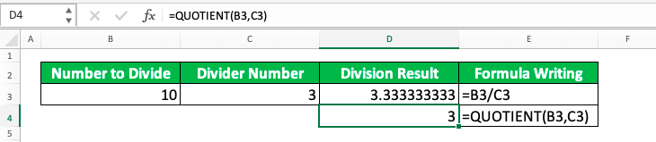
From the example, you can see the difference of results between the normal division formula and QUOTIENT. The normal division formula will give us a division result with the remainder from the process (as you can see in the result’s decimals). QUOTIENT, on the other hand, will give us a division result without its remainder, just the whole number.
Therefore, if you need the type of result that QUOTIENT gives, then don’t hesitate to use the formula!
How to Get the Remainder of a Division Calculation in Excel: The MOD Formula
QUOTIENT will give us a division result without the remainder. Sometimes, however, you probably want the remainder instead without the actual division result. For that, you can use another division related formula in excel, MOD.The way to write MOD is quite similar to QUOTIENT.
= MOD( number_to_divide, divider_number)
Just input the number you want to divide and the divider number into MOD and you are good to go!
Here is the example of the MOD formula in action.
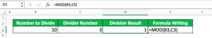
As you can see in the formula writing, the way to write MOD is almost the same as QUOTIENT. We input the number to divide and the divider and get the result we want from it.
The only difference is in the kind of result MOD gives to us as you can see in the example. There, we try to divide 10 with 3. Because the remainder of that division is 1, that is the result we get from MOD.
How to Divide Columns in Excel
It is all easy and fast if we just try to divide a pair of numbers. However, we often need to divide numbers in one column with other numbers in another column.What should we do so we can finish that division calculation much faster? It will surely take much time if we need to write a division formula separately for each pair of numbers.
As a solution for that, we need to know how to divide columns in excel. That can be done by using the copy feature in excel.
To understand better the method to do that, let’s see the explanation through an example below.
Let’s say we have two columns with numbers like this.
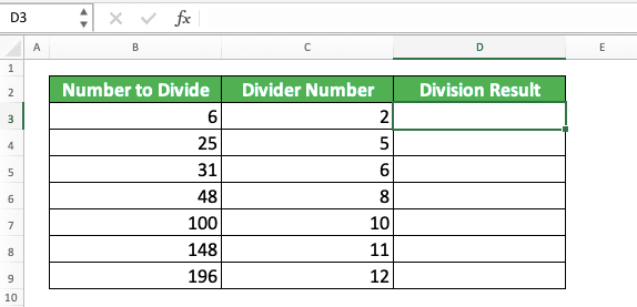
We want to divide all the numbers in the left-most column with their pairs on the right. How can we do that fast?
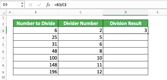
First, we create the division formula for the first pair of numbers from those two columns like this.
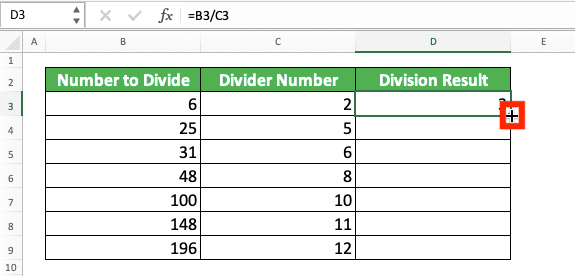
After that’s done, we will just copy down the formula until we get all the division results we need. To do that, we move our pointer to the bottom right of our cell cursor until it becomes a + like this. The cell cursor must already be on the cell where we previously wrote our division formula.
Then, we click and drag our pointer until the bottom of the number pairs from both columns. We will immediately get the columns division results!
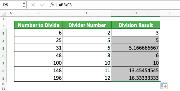
Not too hard, isn’t it? Follow those steps if you need to divide numbers in the columns of your own excel file!
How to Divide a Column by a Number (Constant) in Excel
What if we have a number we constantly want to be the divider for all numbers in a column? For example, we might need to see the production outputs per hour from companies’ factories. Thus, we need to divide the total production outputs per factory by the same precise number of production hours.What do we do? Well, the key here is to differentiate how we input the number to divide and the divider in our division formula.
We need to input the number to divide with its cell reference. Thus, it can move along when we copy our division formula to calculate the whole column numbers.
For the divider, we need to input it either by direct typing or by an absolute cell reference. That way, we can make it constant for each of our division formulas when we do the formula copy process.
If you want to use the absolute cell reference, then you need to add $ symbols for the divider cell reference. We add the $ symbols in front of the column letter and row number (e.g. $A$1 if the divider number is in cell A1). You can do that by typing the symbols directly or by pressing the F4 (Command + T in Mac) button after you input the cell reference.
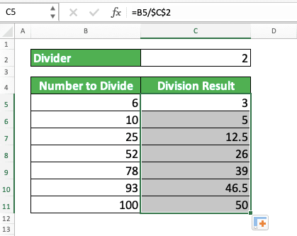
For the example of this column division by a constant, let’s say we have a column of numbers like this.
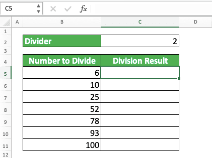
We want to divide all the column numbers using the 2 in cell C2. How do we do that fast?
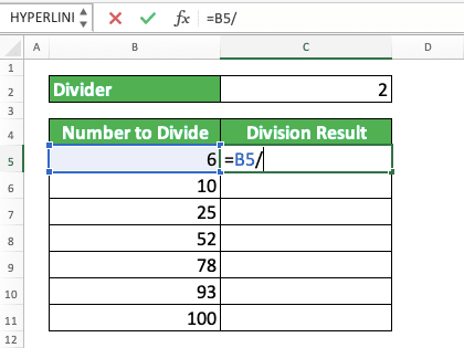
First, we type the division formula for the first number of the column. For that, we input the equal symbol ( = ), the cell reference of the number to divide, and the slash symbol ( / ).
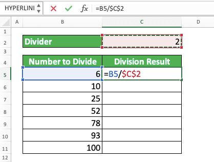
Then, we input the divider by typing it directly or by using the absolute cell reference of cell C2. You can see both methods’ implementation in the example below.
Direct number typing.

Absolute cell reference.
After we finish with the division formula writing, we will copy it down to divide all the column numbers. To do that, place your cell cursor in the cell with the formula. Then, move your pointer to the bottom right of the cell cursor until it becomes a + symbol like this.
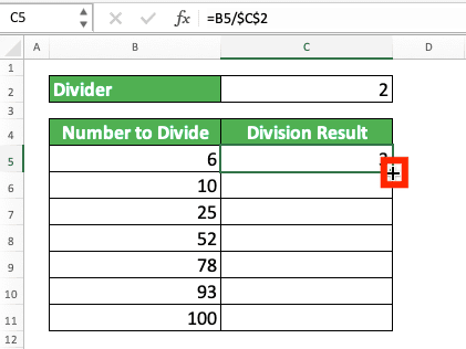
Then, click and drag the pointer until the formula covers the division for all the column numbers. Release the drag and you will get the column and constant division result!
Almost the same as the steps for the columns division, right? Just don’t forget to make the divider input constant by using the methods explained above.
How to Divide a Number with a Percentage
If we want to divide a number with a percentage, that means we want to get the “100%” of the number. This can be like, for example, if we have a discounted price and we want to get the original price.The division formula principle for this is much the same as the usual division formula writing in excel. However, don’t forget to put the percentage as the divider and have the percentage symbol also.
= percentaged_number / percentage%
From this writing, we will get the 100% of the number we divide.
For example, take a look at the screenshot below.
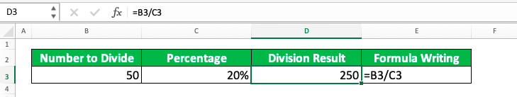
As you can see in the example, we divide the 50 we have with the 20%. As a result, we get the 100% of the 50 (we assume the 50 is the 20% of the “original” number), which is 250.
We don’t need to input a percentage again in our formula writing because the number in our cell already has it. However, if we type the number directly, then we mustn’t forget to add the symbol to get the correct result.
Note that you can also change the percentage with its decimal equivalent (e.g. 20% is the same as 0.2 or 50% is the same as 0.5). You will get the same result either way.
How to Handle a #DIV/0 Error
In division calculation, you cannot divide any number with zero as the result will be undefined. This also applies to excel as any number you divide with zero will result in a #DIV/0 error.However, you may sometimes unintentionally get this kind of error.
Probably, you have many numbers in your columns and you don’t know that few dividers there are zero. As a result, you will get some #DIV/0 errors from your division calculation.
This isn’t good especially if you want to process the division results further. Those errors can cause other further errors and you won’t get the end results you want from your excel work.
So, what to do to anticipate the #DIV/0 error in your division calculation in excel? You can use the IFERROR formula which can then change your error with an alternative value.
To use it with your division formula writing, the general writing form can be such as this.
= IFERROR( number_to_divide / divider_number , alternative_value)
Input your division formula as the first input of IFERROR and the alternative value as the next one. You can give any alternative value you want as the substitute for the #DIV/0 error.
With this writing, if your division formula results in an error, then IFERROR will automatically change it with its alternative value (if it doesn’t result in an error, then IFERROR will produce your division formula result without any change to it)!
As an example of this writing implementation, see the screenshot below.
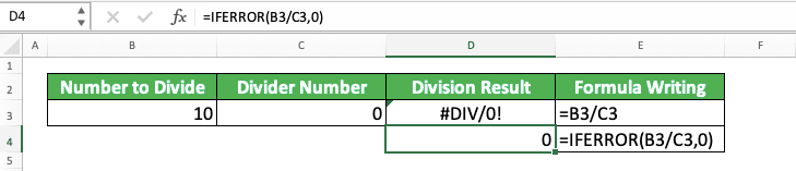
In the example, we can see the comparison of the results between a division formula only and the one with IFERROR.
When we produce a #DIV/0 error because the divider is 0, IFERROR will change the error with the alternative value. If we don’t put an IFERROR, then the error will become the end result of our formula writing.
Therefore, if you need to anticipate errors from your division formula, then don’t hesitate to use IFERROR! That way, you won’t produce errors that can derail your data processing in excel.
Exercise
After you have learned how to divide in excel using various methods, now let’s do an exercise. This is so you can understand the usage of the methods deeper.Download the exercise file and answer the questions below. Download the answer key file if you have done the exercise and want to check your answers.
The link to the exercise file:
Download here
Questions
- How many productions per machine are needed to achieve the production target this month? Make the result to have 3 decimal digits (look at the additional notes part of this tutorial if you don’t know how to round your answer!)
- How many productions per machine to achieve the production target if the target is distributed evenly? Use QUOTIENT to answer!
- How many production target remainder is still not distributed to any machine if the target is distributed evenly? Use MOD to answer!
The link to the answer key file:
Download here
Additional Note
To increase/decrease the decimal digits from your division formula, use the increase decimal/decrease decimal menu from the Home tab. Place your cursor first on the cell where the result is to use it.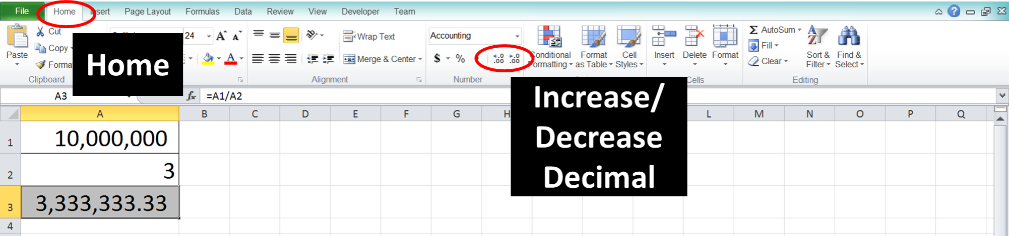
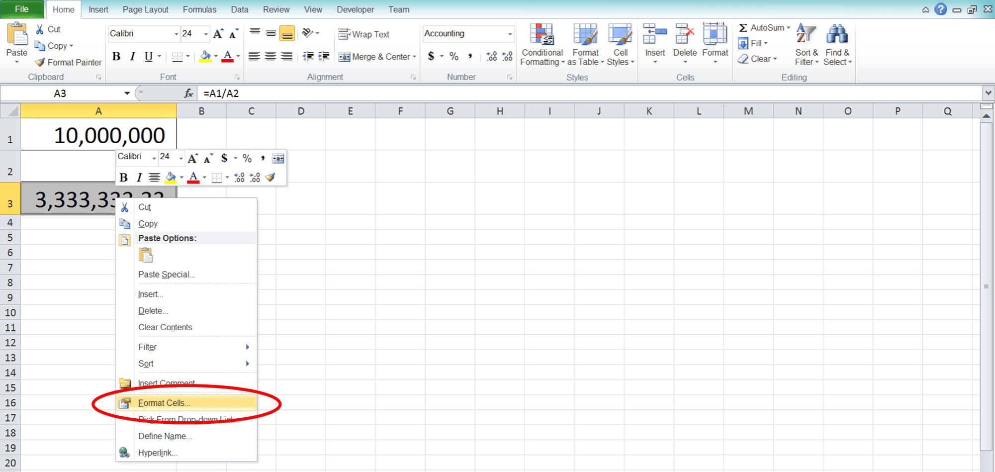
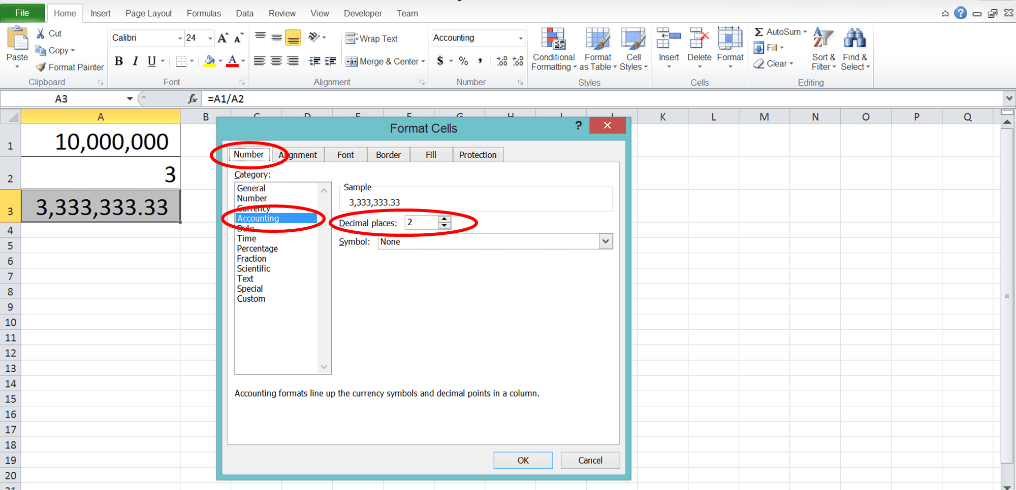
Or right-click after placing the cursor then click Format Cells. Then, in the Number Tab, choose Number and replace the Decimal Places value with the number of decimals you want. Last but not least, click OK.
But, it is important to remember that this method only changes the decimal look of your number, not its value. If you want to change the value too, then you need to practice the actual excel rounding process. The tutorial to do it is provided too in this blog!
Related tutorials you should learn: