How to Create a Drop-down List in Excel

In this tutorial, you will learn how to create a drop-down list in excel in the right way.

When working in excel, we sometimes need to restrict the inputs in some cells so they don’t go out of hand. We might need that so our data processing will be much easier later or so there won’t be any crazy input.

One of the most popular choices to restrict input in excel is to use the drop-down feature. We can create various kinds of drop-down, from the simple one to the more complicated one. It purely depends on our needs which kind of drop-down we should use.

Want to master the creation of a drop-down list in excel so you can create the best one for yourself? Learn from this tutorial until its last part!

Disclaimer: This post may contain affiliate links from which we earn commission from qualifying purchases/actions at no additional cost for you. Learn more

Want to work faster and easier in Excel? Install and use Excel add-ins! Read this article to know the best Excel add-ins to use according to us!

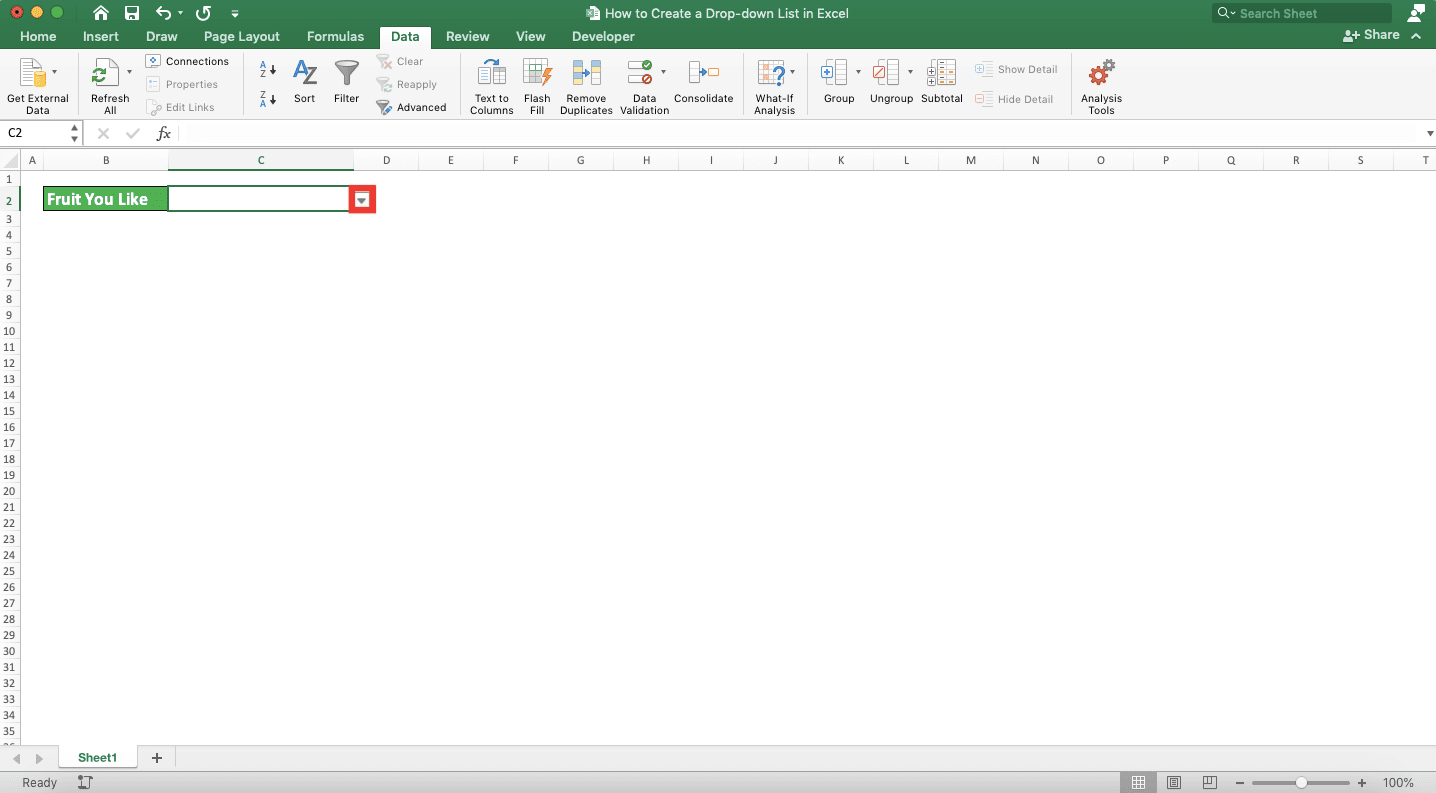
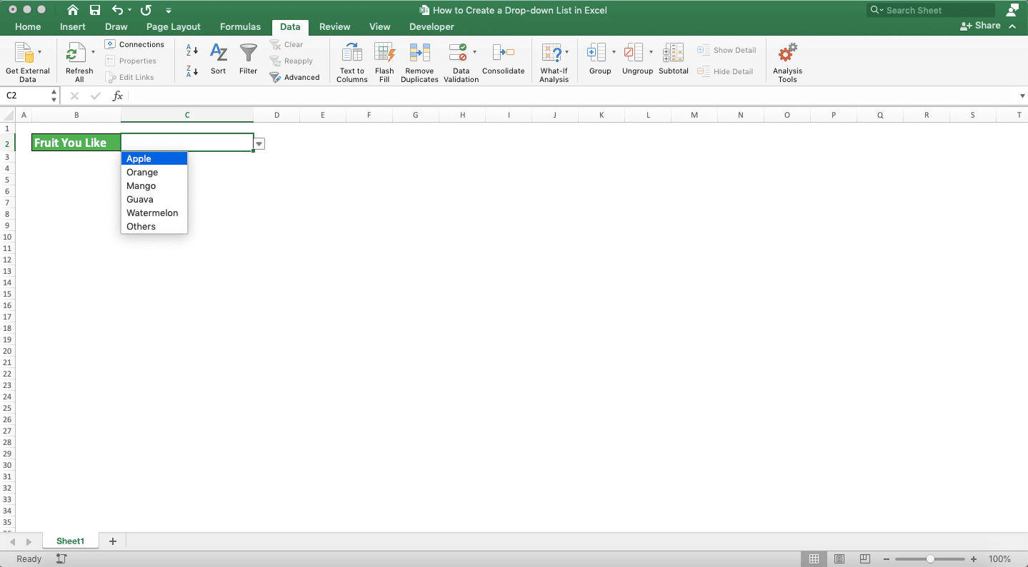
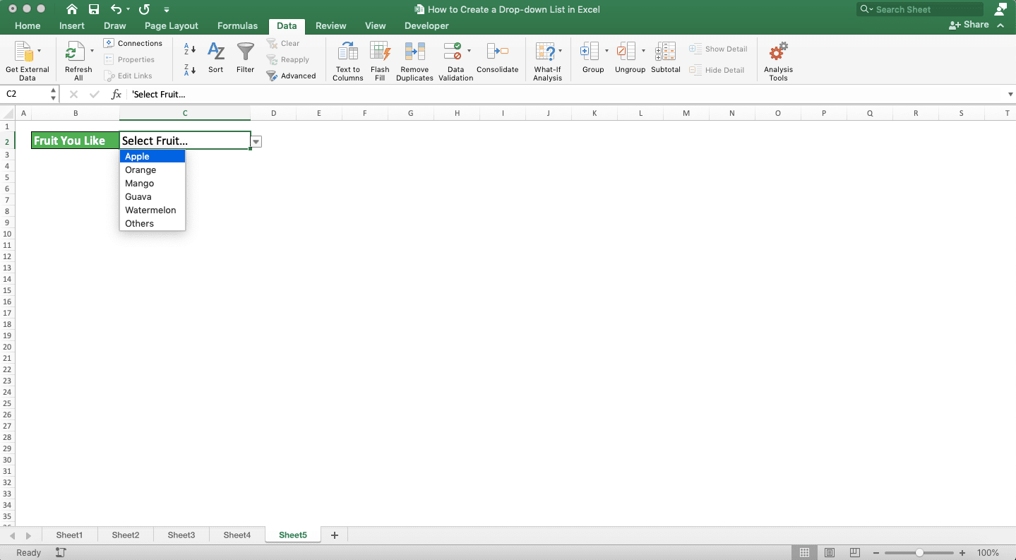
How to Create a Drop-down List in Excel Manually

Let’s start the tutorial by discussing about how to create the most basic form of drop-down list in excel. It is a drop-down list with choices that we type manually into the drop-down.

The process to create this kind of drop-down list in excel isn’t too hard. Here is the step-by-step to do it.

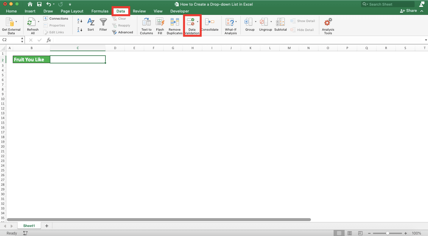
1. Select the cell where you want to create a drop-down list
   
   
   
   
2. Go to the Data tab and click the Data Validation button there
   
   
   
   
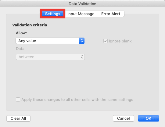
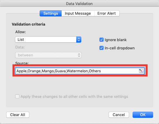
3. In the dialog box that shows up, make sure you are in the Settings tab
   
   
   
   
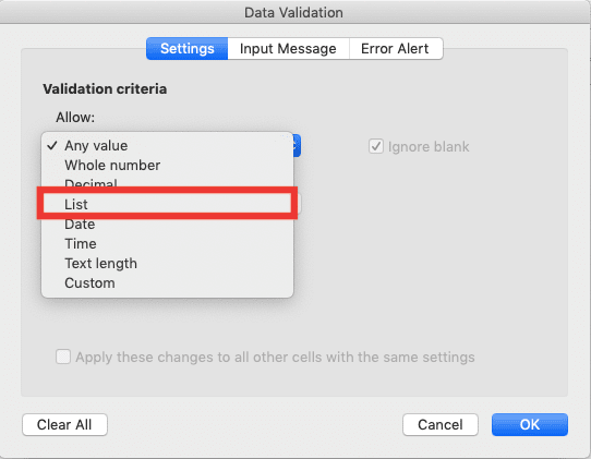
4. In the Settings tab, click the Allow dropdown and select List
   
   
   
   
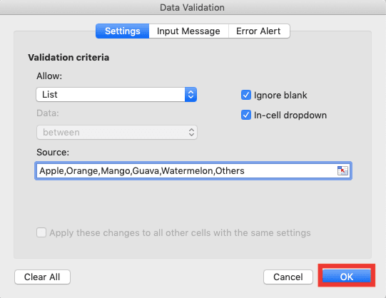
5. In the source text box that shows up, type the choices you want for your drop-down list. Separate each of the choices you type with a comma sign ( , )
   
   
   
   
6. After you have typed all the choices you want for your drop-down list, click OK
   
   
   
   
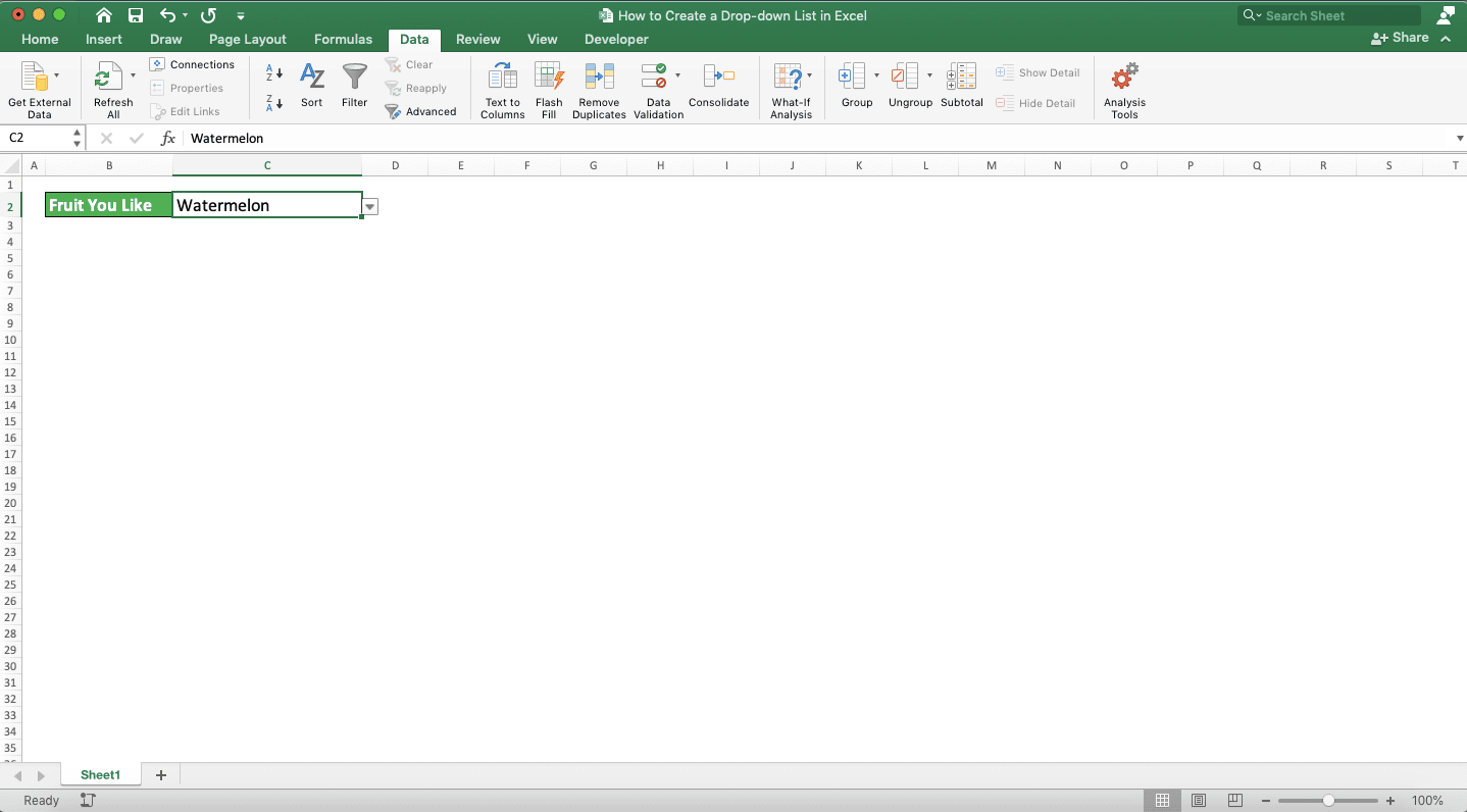
7. Done! Now, your cell should show a drop-down button when you select it. When you click the drop-down button, you can choose an input for the cell from a drop-down list
   
   
   
   
   
   
   
   

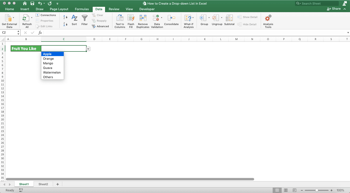
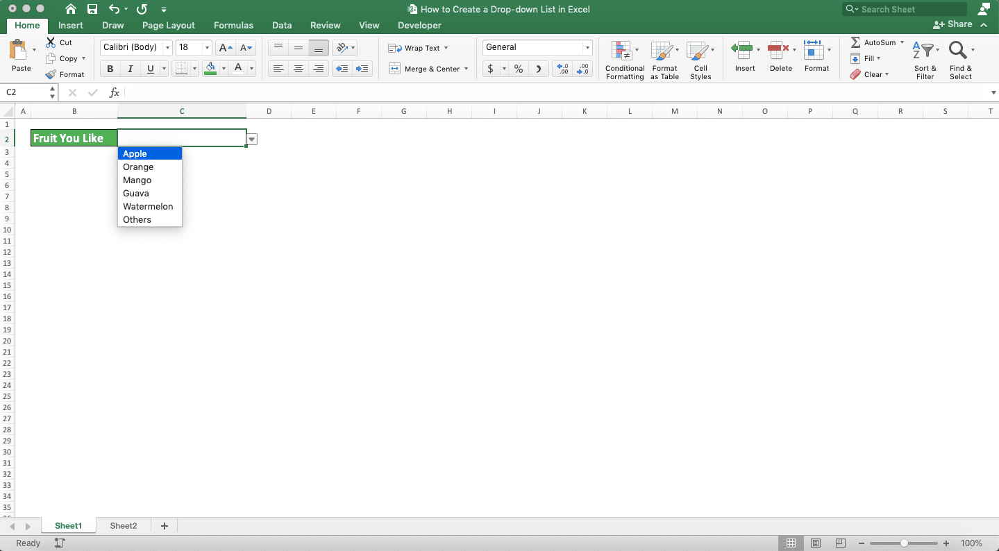
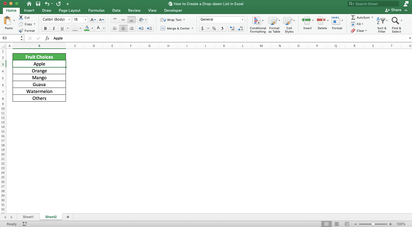
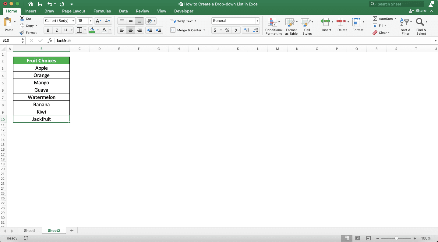
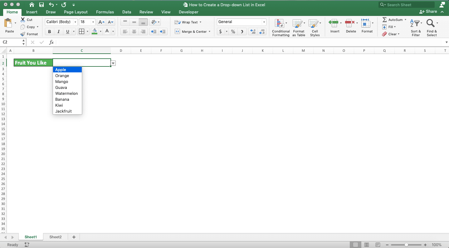
How to Create a Drop-down List in Excel with Choices from a Cell Range

Already have your drop-down choices in a cell range and want to input from there instead of typing them manually? You can do that easily in the drop-down source text box in the data validation dialog box.

On the right side of the source text box, you might notice that there is a button there you can click. Just click on it if you want to input a cell range as the source of your drop-down choices.



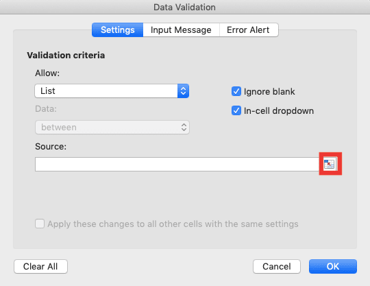
In the dialog box that shows up after you click the button, input your cell range by dragging on it. Excel will automatically input the cell range coordinate you drag.



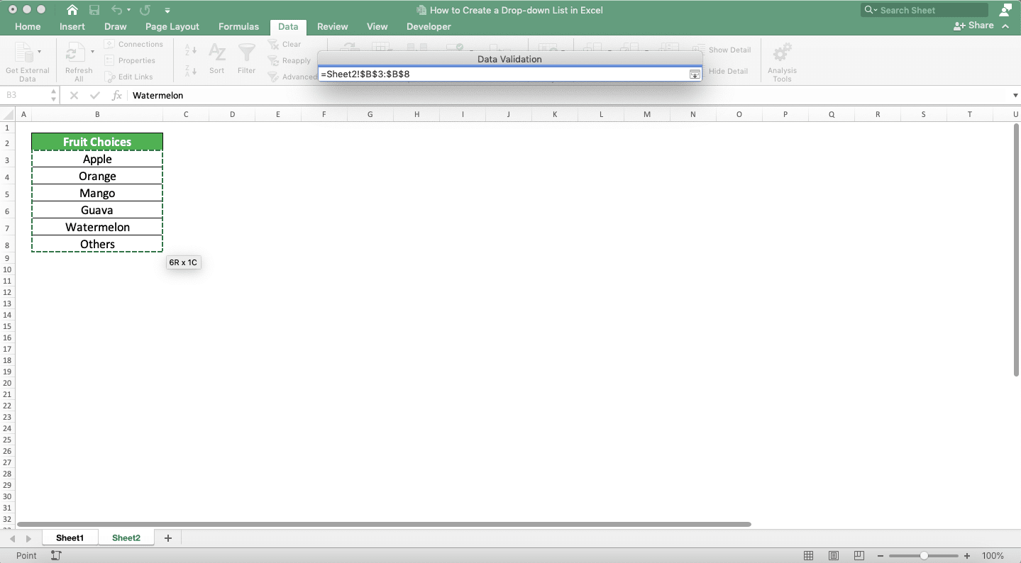
Click the button in the text box of the dialog box after you finish inputting the cell range.



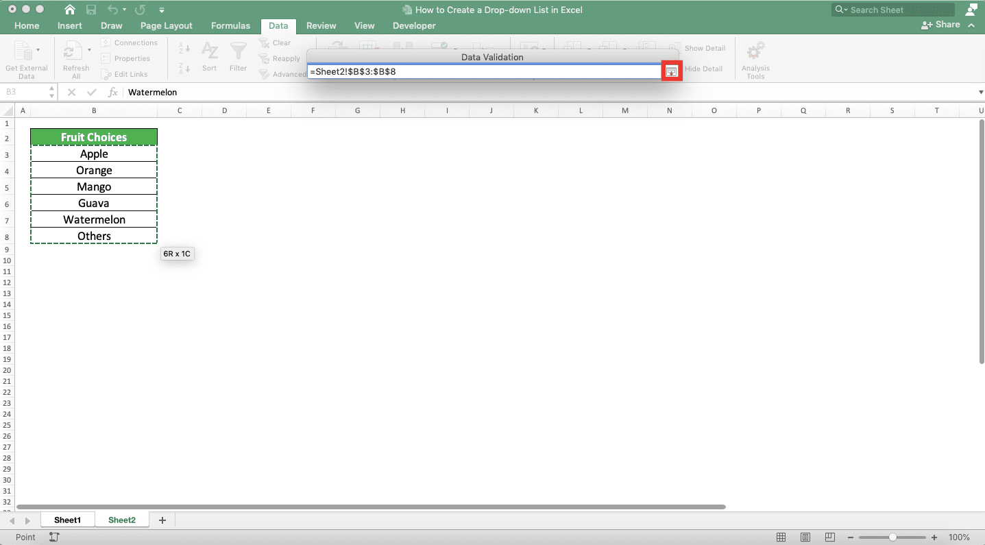
Then, click OK. Now, you have created a drop-down with the source of the choices from the cell range you set earlier!

How to Add/Remove Choices from a Drop-down List in Excel (Edit Drop-down List)

Need to edit the choices in the drop-down you have made? First, check whether you input them by typing them manually or by inputting a cell range.



If you typed the drop-down choices manually, then you need to go back to your cell’s data validation dialog box. In the source text box, you can edit your drop-down choices directly by deleting, re-typing, or typing new ones.



If you input them from a cell range, then you can go to the cell range and edit the choices there. Re-type the choices which you want to edit.

If you want to delete one/some of them, highlight the choice cells and then right-click on them. Choose Delete… to show a Delete dialog box.



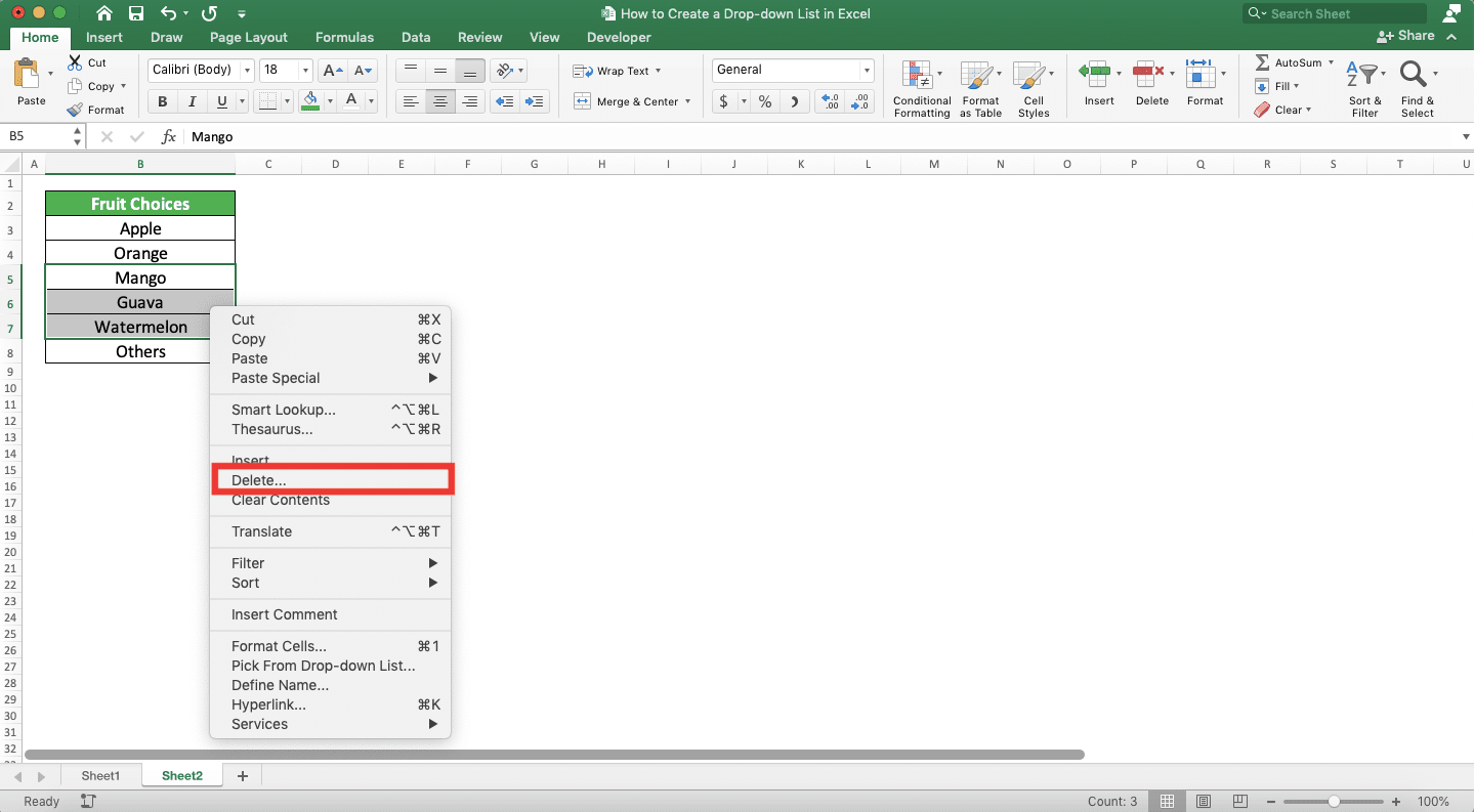
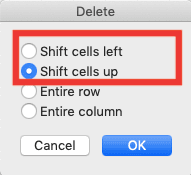
Choose Shift Cells Up in the dialog box if you want to move up the cells below after you delete. Choose Shift Cells Left if you want to move the cells on the right to the left after you delete.



You have removed the choices you highlight from your dropdown!

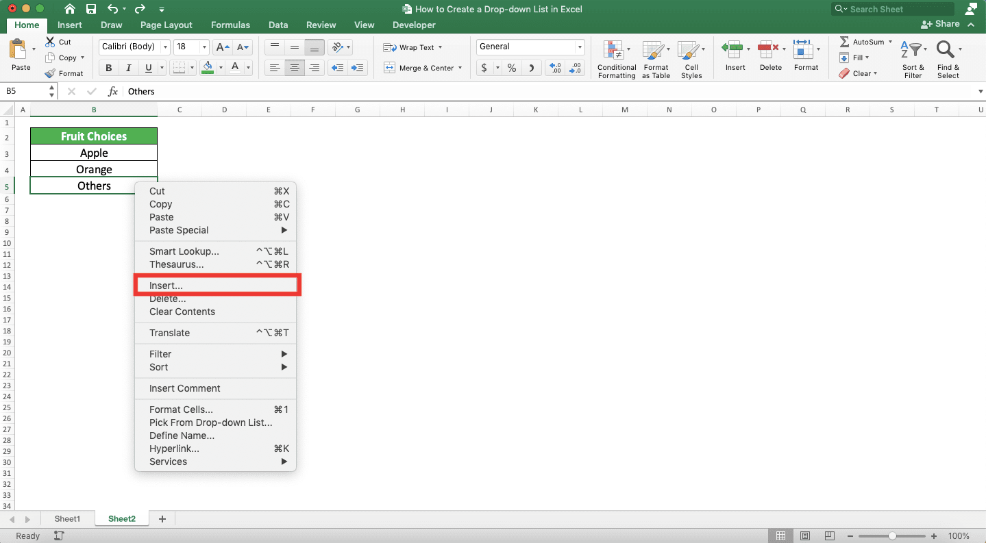
If you want to add the choices in the cell range, then do the opposite. Highlight the number of cells in the cell range which corresponds to the number of choices you want to add. Then, right-click on them and choose Insert… to show an Insert dialog box.



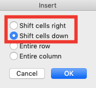
Choose Shift Cells Down if you want to move down the cells you highlight to insert cells for your new choices. Choose Shift Cells Right if you want to move them to the right. The one you should choose should depend on the cell range form you have.



Insert the cells and type your drop-down additional choices on the empty cells you have just inserted. After that, your drop-down should contain those choices in its list!

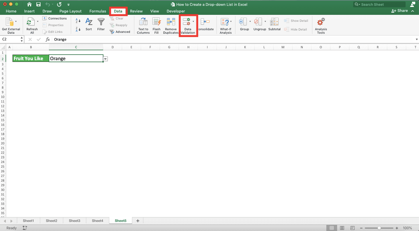
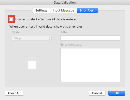
How to Allow Other Entries in the Cell with a Drop-down List

By default, you cannot input anything other than the dropdown choices if your cell has a drop-down. If you need to allow other inputs, however, then you need to set the allowance in the cell’s data validation settings.

To allow that, highlight the cell with the drop-down, go to the Data tab, and click the Data Validation button. In the Data Validation dialog box, go to the Error Alert tab. Then, remove the checkmark in the “Show error alert after invalid data is entered” check box by clicking on it.



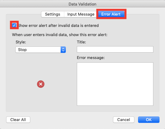
Click OK after that. Now, your cell will allow inputs other than the ones in its dropdown choices!

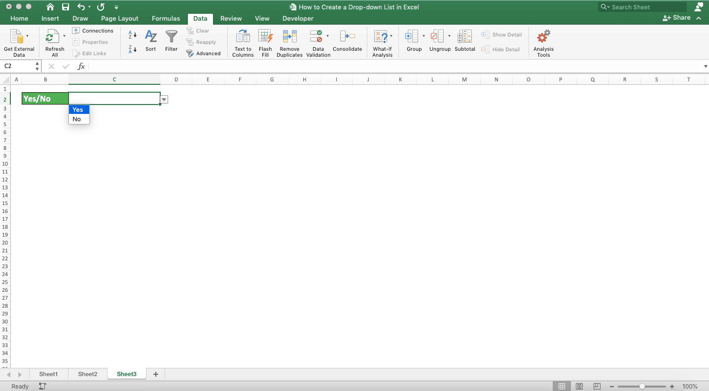
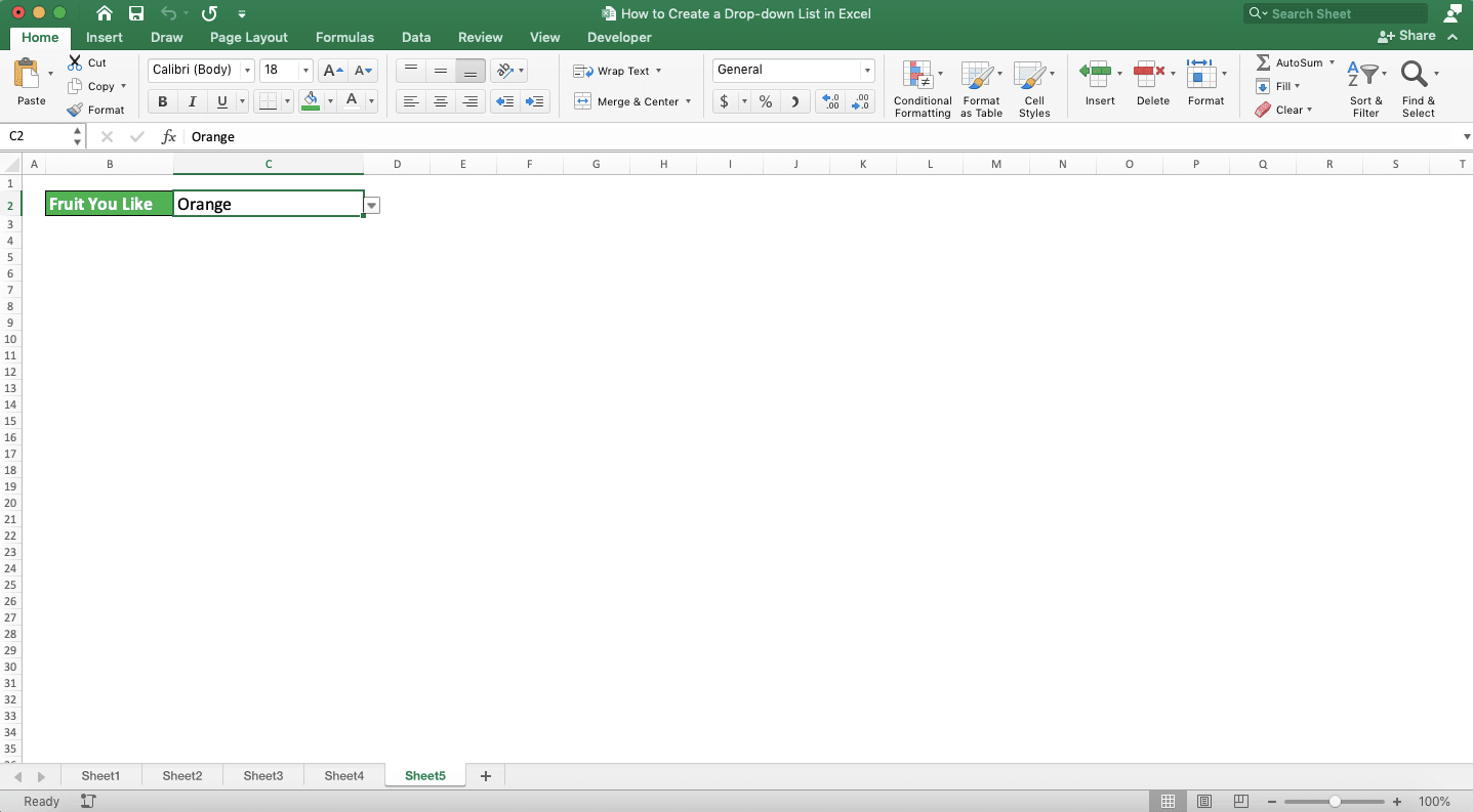
How to Create a Yes No Drop-down List in Excel

To create a yes/no drop-down list in your cell, input yes and no as your drop-down choices. You can type them directly in your drop-down list source text box or input them via a cell range.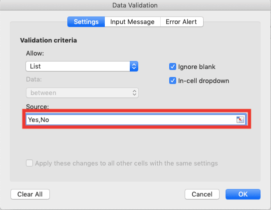



Do that and you should have a drop-down list in your cell that contains yes and no choices.

How to Create a Conditional/Dependent Drop-down List in Excel

From this tutorial part, we will begin the discussion to create a more complex drop-down list in excel. The first one to discuss is creating a conditional/dependent drop-down list in your cell.

You may sometimes need to create a drop-down list which choices depends on another cell value. A simple example of this is city drop-down choices that might depend on the country cell value. If you choose a different country, then the city drop-down choices should change.



How to create something like that in excel? To create this kind of drop-down list, we should use the combination of INDIRECT, SUBSTITUTE, and cell range names.

We name each cell range which contains the scenarios and the drop-down choices we have for each scenario (country names and city names for each country for the case of countries and cities). Then, we use the scenario name as the source in the cell which value our other drop-down choices depend on. Finally, we combine INDIRECT and SUBSTITUTE to convert the cell value to the named cell range for the drop-down choices.

Got confused with the explanation? Follow the discussion of the example below to understand the concept better!

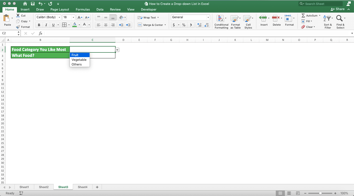
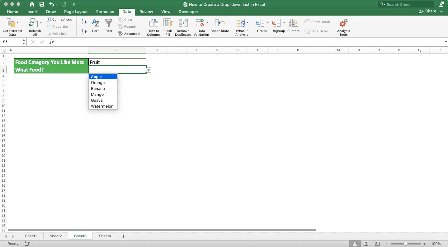
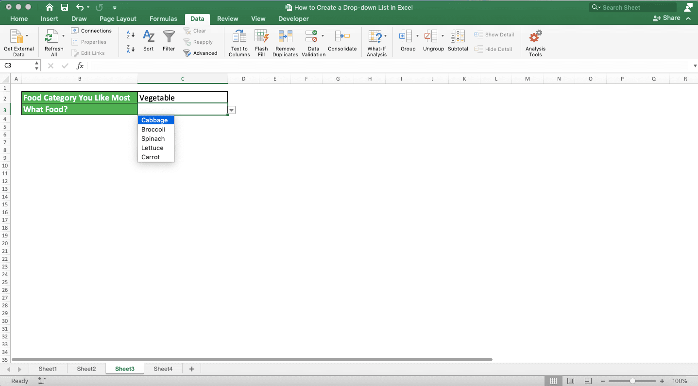
Let’s say we have two drop-downs we want to create in our cells below. The drop-down choices for the “What Food?” depend on the food category value above it.



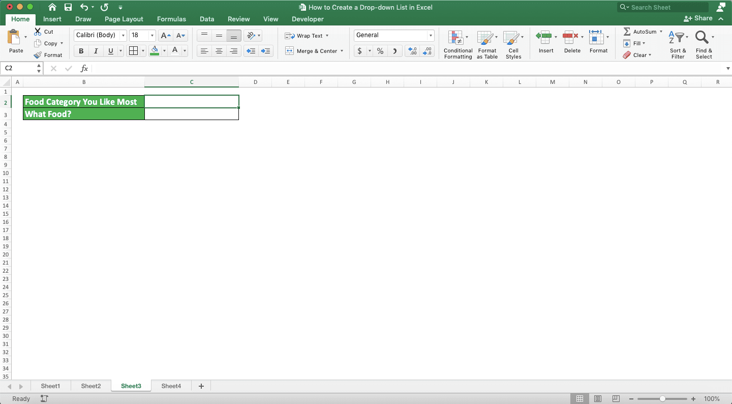
In a different sheet, we have the references for the food categories and their food choices.



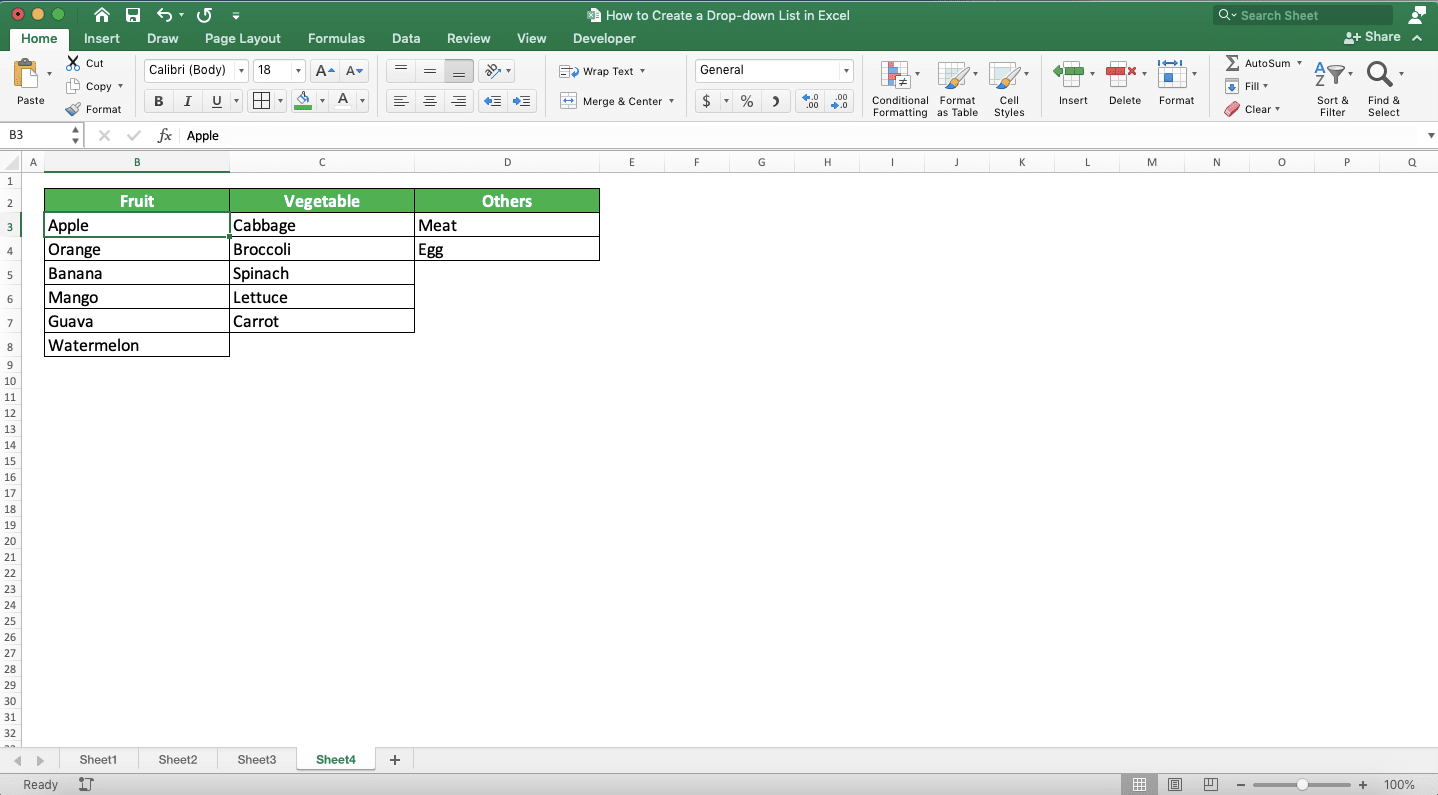
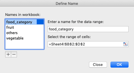
What should we do to create two drop-downs? Well, first we name the cell ranges that we need for our drop-downs in the reference sheet. In this example, we should name the cell ranges for the food category and food choices in each category. The name of the food choices cell ranges should be the same as the name of their food category.

We have four names after we name all the cell ranges we need in the example.



After we finish the names, we go back to the sheet where we want to create our drop-downs. In the food category cell, we create a drop-down with our “food_category” name as its data validation source. We do that by typing “=food_category” in the data validation source text box.



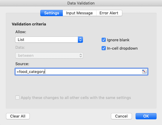
Do that and the cell drop-down choices will become the same as the values in our food_category cell range.



Next, we create the dropdown for our second cell. For this, we write the combination of INDIRECT and SUBSTITUTE in its data validation source text box.



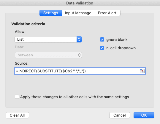
We use SUBSTITUTE inside our INDIRECT here since we want to anticipate spaces in our cell value. Since we cannot name our cell range with spaces, we should substitute them with underscores ( _ ). SUBSTITUTE will handle the substitution process for us in the data validation source.

The INDIRECT here is important because it can convert text into a formula reference. Without using INDIRECT, excel won’t recognize our cell value as a cell range name.

We do all that and we will get a conditional/dependent drop-down in our cell! Now, whenever we change the cell value that becomes our drop-down reference, our drop-down choices change too.

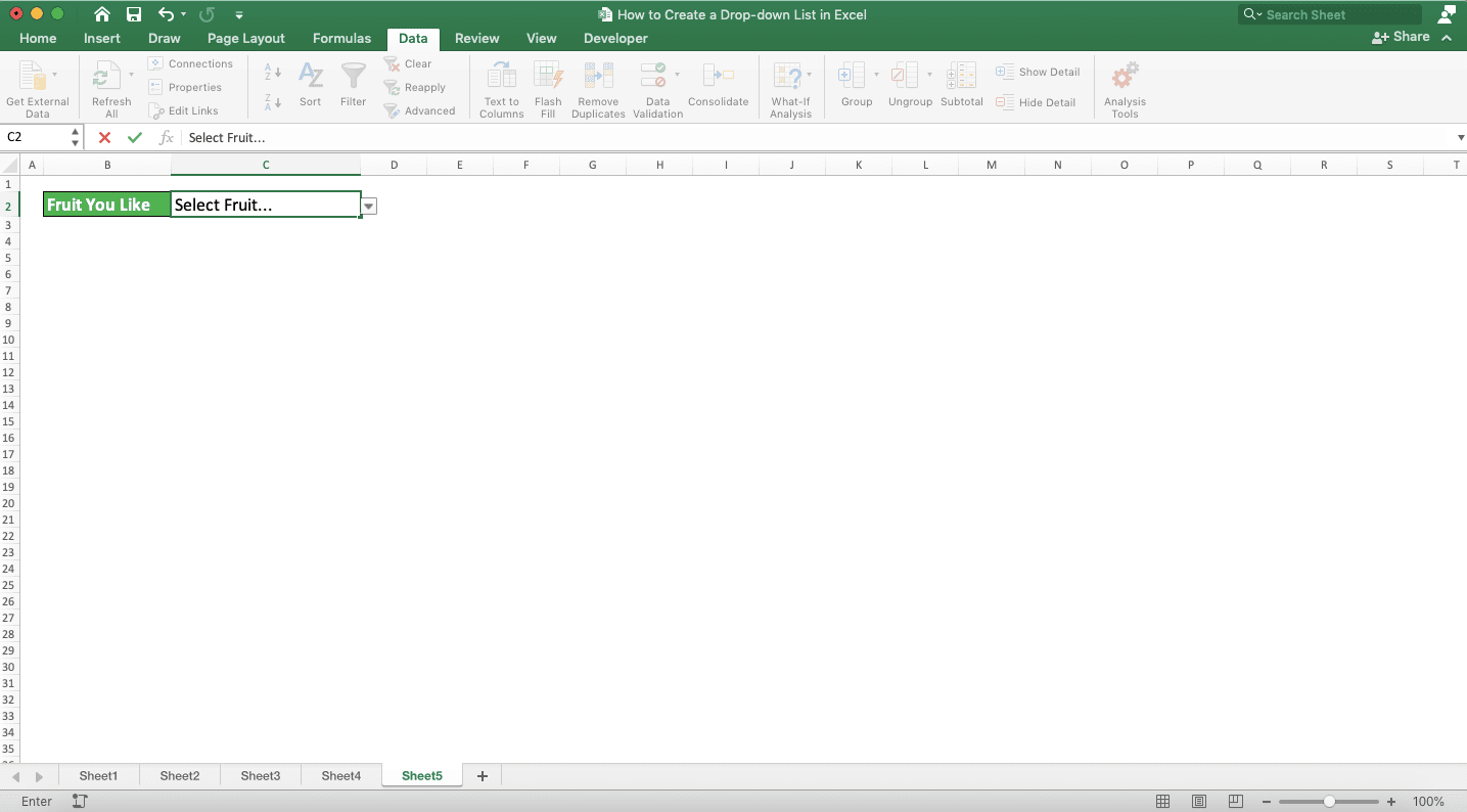
How to Create a Drop-down List with a Default Value in Excel

Need to have a default value for your drop-down before a person selects a choice from it? You need to create your drop-down first for this. After your drop-down is ready, you can follow these steps.

1. Highlight the cell where your drop-down is
   
   
   
   
2. Go to the data validation dialog box by going to the Data tab and click the Data Validation button there
   
   
   
   
3. Allow other entries in your cell by unchecking the check box in the Error Alert tab (click on it if it has a checkmark). Then, click OK
   
   
   
   
4. Type the default value you want for the drop-down
   
   
   
   
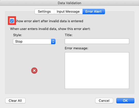
5. Go back to the data validation dialog box to check the checkbox in the Error Alert tab again (click on the checkbox). Click OK
   
   
   
   
6. Done! Now, the cell with the drop-down shows up a default value before we select a drop-down choice there
   
   
   
   

How to Create a Dynamic Drop-down List in Excel

When we refer to a cell range as the source of our drop-down choices, we may need a dynamic reference. This means when we input new data to the cell range, we want the dropdown choices to automatically include it.

We can do that but we cannot just input the cell range as the dropdown choices source. We should use the combination of OFFSET and COUNTA when we input the source of the dropdown choices.



Here is the general writing form of the OFFSET and COUNTA combination for the dynamic drop-down choices source.



This formula writing assumes you have a column cell range for your drop-down list. If you have a row cell range, you can swap the position of COUNTA and 1 there. The 1 input here means that OFFSET won’t expand the cell range horizontally, only vertically (for a column cell range).

OFFSET can expand the cell we input depending on the other inputs we give to it. We write COUNTA in the OFFSET input part which asks how many cells it should expand our cell vertically. In the other inputs, we input something that makes the cell in OFFSET not move (0 and 0 for the inputs of how far we want the cell to move).

As COUNTA counts all data in its cell range, OFFSET will expand our cell depending on the data it has! Therefore, we should input our cell range to COUNTA by including the cells where we will input our new data too.

Here is an implementation example of the dynamic drop-down list concept by using the OFFSET and COUNTA combination. Let’s say we have this drop-down below.



The drop-down choices source comes from the cell range in another sheet.



To make the drop-down includes new data we give to the cell range later, we write this as its source.



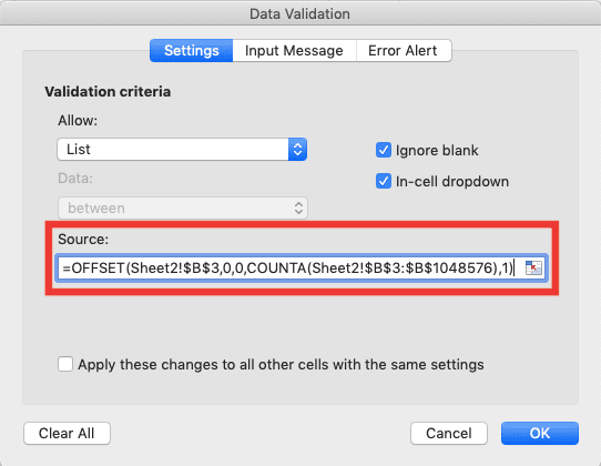
In the OFFSET, we input the cell coordinate where our first drop-down choice is as the first input. In other OFFSET inputs besides COUNTA, we input 0, 0, and 1 as we discussed previously.

In the COUNTA, we input the cell range that we expand to include all cells where we will input new data. Thus, we input the cell range from the first cell in our cell range until the last row in the worksheet!

As a result of the OFFSET and COUNTA combination, we can update our drop-down choices easily. Just enter new data in its cell range source and we are good to go!

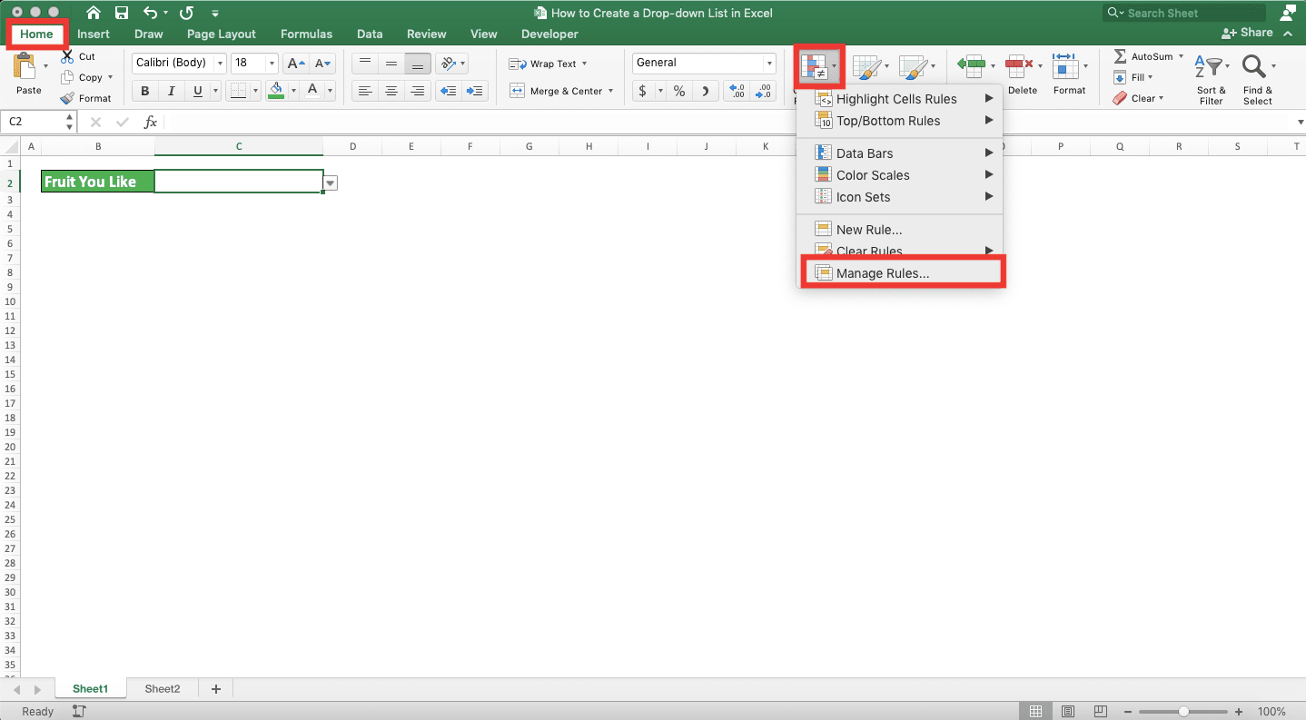
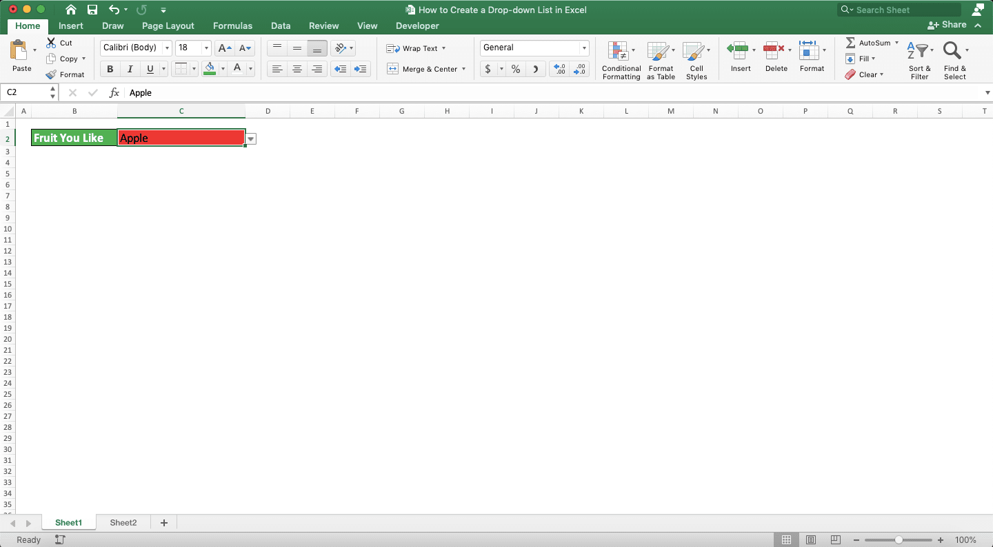
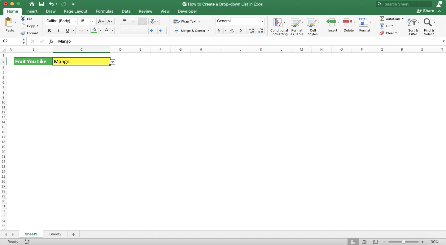
How to Create a Drop-down List with Color in Excel

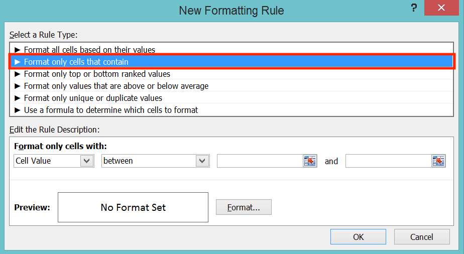
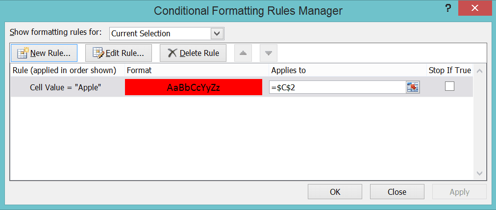
Want to make your cell shows a specific color when you pick a specific choice from your drop-down list? We can create something like that by using the Conditional Formatting feature in excel.

Just set the rules in your cell’s conditional formatting that give each choice in your drop-down a certain color. To do that, first, highlight the cell with the drop-down list. Then, go to the Home tab, click the Conditional Formatting button dropdown, and choose Manage Rules….



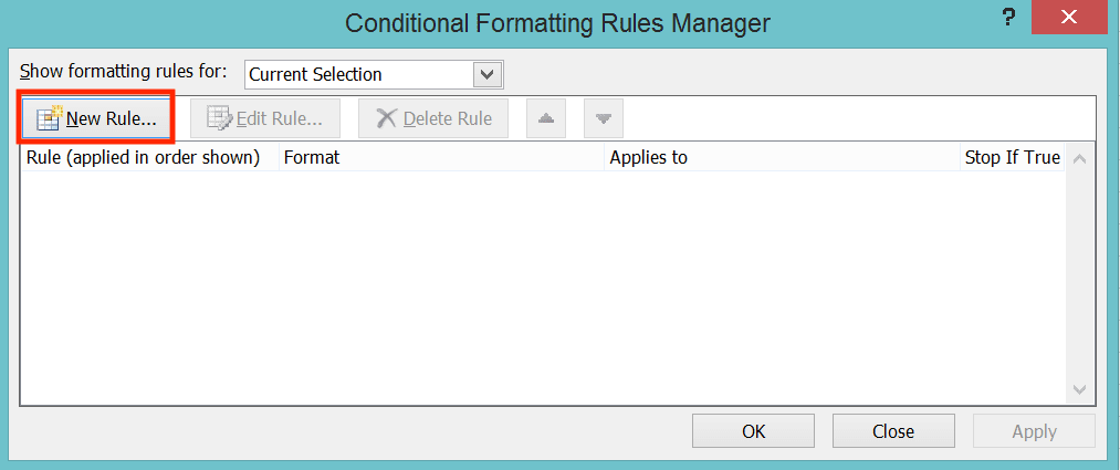
In the dialog box that shows up, click the New Rule… Button.



Choose “Format only cells that contain” in the Select a Rule Type box.



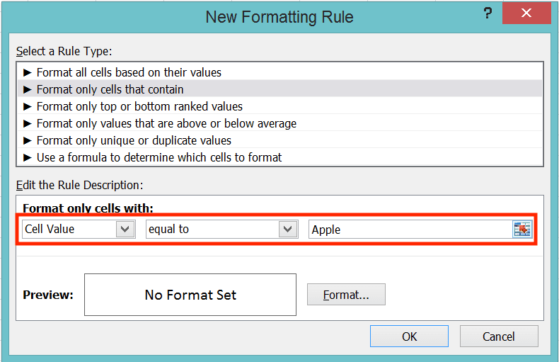
In the part below the Select a Rule Type box, choose “Cell Value” and “equal to” in the dropdowns. Then, input the first choice of your drop-down either by typing it directly or by using a cell coordinate.



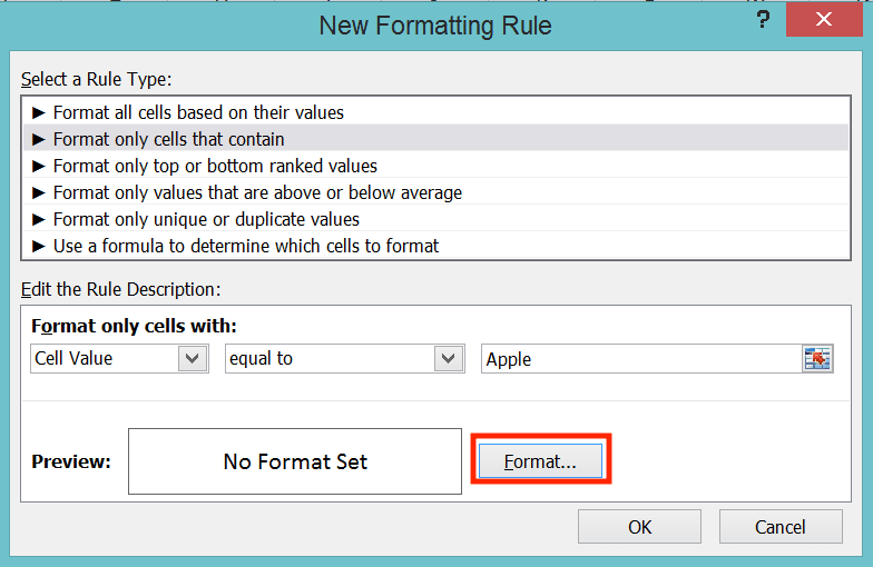
Next, click the Format… button below.



There will be a dialog box where you can format your cell if it contains the drop-down first choice. As you want to color it, go to the Fill tab and choose the color you want there.



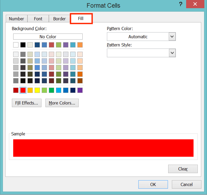
Click OK and then OK again. You have added the color rule for your first drop-down choice!



Click the New Rule… button again. Now, repeat the steps above until you have given colors to all your drop-down choices.



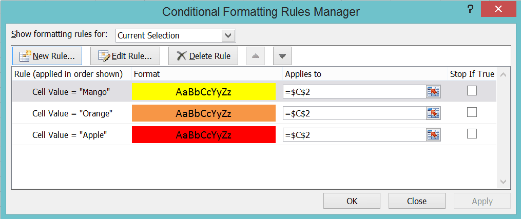
Click OK after you have done that. Now, your cell will change its color according to the drop-down choice you choose!

How to Manage a Drop-down List Font Size in Excel

The font size problem in a drop-down list usually happens if you use a Windows computer. You may sometimes find that the font size of your drop-down choices is too small to read.



How to change the drop-down choices font size? There are two things you can adjust when you need to change your drop-down choices font size.

• The font size in the text in the same worksheet as the drop-down. Try to make it smaller so your drop-down font size can stand out more
• The zoom level of your worksheet. Try to zoom in so you can read the font in your drop-down choices

Unfortunately, you cannot change the font size in your drop-down list directly. Therefore, try to play with the two variables we mentioned so you can get the right font size for yourself!

Drop-down List Shortcut in Excel

Need to select a choice from the drop-down in your cell without using a mouse?

You can press Alt + down (Option + down in Mac) to open the drop-down list in your cell. After that, just press the up or down button to toggle between the drop-down choices.

After you highlight the drop-down choice you want, press enter. You have inputted your cell from the drop-down list without using a mouse!

How to Remove a Drop-down List in Excel

Removing a drop-down list from your cell in excel is quite easy.

Just highlight your cell and open the Data Validation dialog box (go to the Data tab and click the Data Validation button there).

In the dialog box, click the Allow dropdown and choose Any Value.



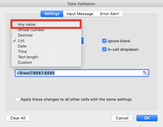
Then, click OK. You have removed the drop-down list in your cell!

Exercise

After you have learned how to create a drop-down list in excel, now it is time to do some exercise. This is so you can understand what you have just learned more practically.

Download the exercise file from the following link and do the instructions below. Download the answer key file if you have done the exercise and want to check your answers!

Link to the exercise file:
Download here

Instructions

Do each instruction in the appropriate gray-colored cell!

1. Create a drop-down from the choices in column 1!
2. Create a drop-down from the choices in column 2 using the OFFSET and COUNTA combination method! Add F, G, and H to column 2. Do they also automatically appear as your cell’s dropdown choices?
3. Create a drop-down from the choices in column 3! Set the cell so it will color itself to your choice color when you pick a choice from its drop-down!

Link to the answer key file:
Download here

Additional Note

INDIRECT and conditional formatting aren’t case-sensitive when running their functions in excel.



Related tutorials you should learn: