How to Use MATCH Formula in Excel: Function, Example, and Writing Steps

In this tutorial, you will learn how to use the MATCH formula in excel completely. MATCH can help you to find the location of data in a specific column/row.

Disclaimer: This post may contain affiliate links from which we earn commission from qualifying purchases/actions at no additional cost for you. Learn more

Want to work faster and easier in Excel? Install and use Excel add-ins! Read this article to know the best Excel add-ins to use according to us!

MATCH Function in Excel

MATCH can help you find data position in a row/column.

MATCH Result

MATCH produces a number that represents the position of data we look for in a particular row/column.

Excel Version From Which We Can Start Using MATCH

We can use MATCH since excel 2003.

The Way to Write It and Its Input

The general form of MATCH writing in excel is as follows



You can see the explanation for the inputs below.

• lookup_value = data you want to look up the position of in an excel row/column
• lookup_array = the row/column cell range where we want to look for the data position
• match_type = optional. The lookup method you want to use. You can see its possible inputs and the explanation for each of the inputs in the table below.
  
  

  Input	Lookup Nature	Explanation
  -1	Approximate	First, MATCH will try to find an exact match for your data. If it doesn’t find it, then it will look for smaller value data closest to the data you want. If you use this input, then your row/column cell range must be sorted in ascending order.
  0	Match	First, MATCH will try to find an exact match for your data. If not found, then it will produce a #N/A error.
  1	Approximate	First, MATCH will try to find an exact match for your data. If it doesn’t find it, then it will look for data with larger value closest to the data you want. If you use this input, then your row/column cell range must be sorted in descending order.

  
  
  The 1 or -1 lookup method input will only be useful if the data you want to find is a number. If you don’t give input here, then MATCH will assume you use the lookup method of 1.

Example of Usage and Result

The following is a MATCH’s implementation example in excel and the explanation of the example.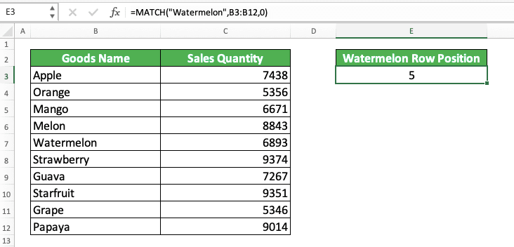



In the screenshot above, we can see how we write a MATCH formula in the formula bar. The writing produces the position of the “Watermelon” word we look for, which is 5.

The data we look for in the example is a text. Thus, we input 0 or an exact match for the data lookup method input part. If we use -1 or 1, then MATCH can produce an error because the data we look for isn’t a number.



Remember that the cell range input in MATCH must be only one row/column, like what we input in the example. If you input more than one row/column, then MATCH can produce a #N/A error.

Writing Steps

After reading and understanding the MATCH implementation example, we will discuss the MATCH writing steps in detail next. Learn this part so you can understand much more about how to use the MATCH formula in excel!

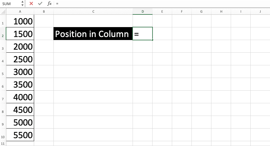
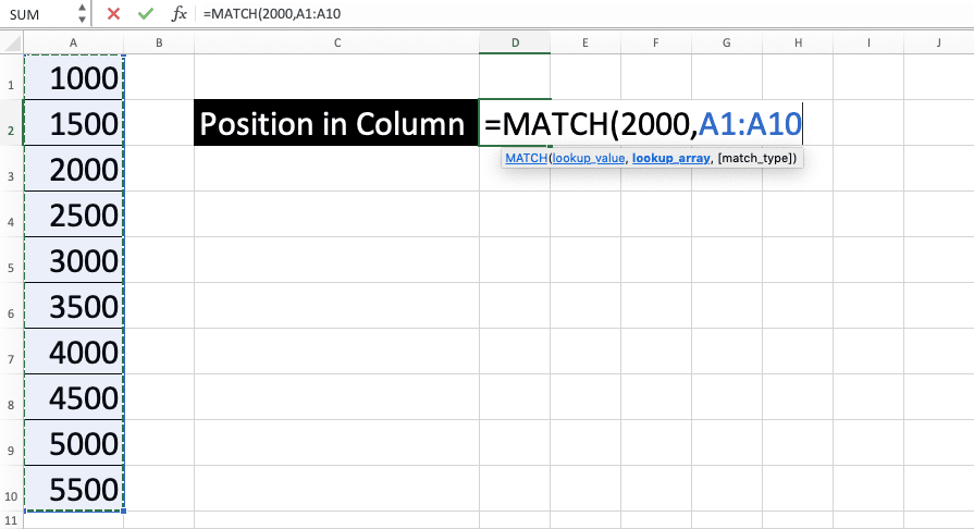
1. Type an equal sign ( = ) in the cell where you want to put the MATCH result
   
   
   
   
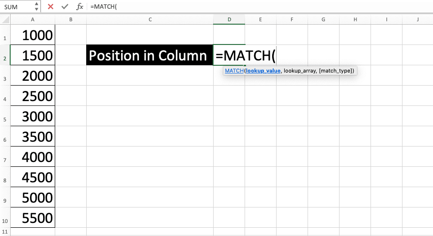
2. Type MATCH (can be with large and small letters) and an open bracket sign after =
   
   
   
   
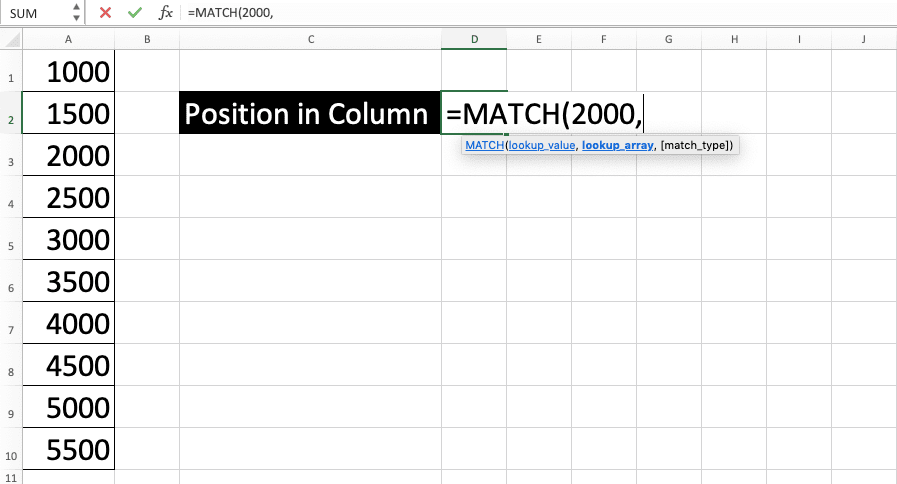
3. Input the data you want to find the position of or the cell coordinate where that data is. Then, type a comma sign ( , )
   
   
   
   
4. Input the row/column cell range where you want to get your data position in
   
   
   
   
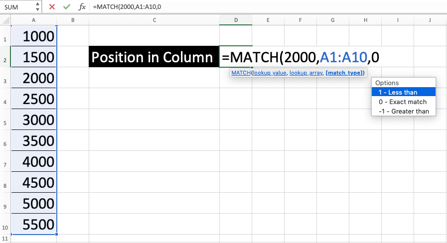
5. Optional: Type a comma sign. After that, input the number that represents the data lookup method you want to use, -1/0/1. Read the explanation on the meaning of each number in the previous part’s table of this tutorial.
   
   
   
   
6. Type a close bracket sign
   
   
   
   
7. Press Enter
8. Done!
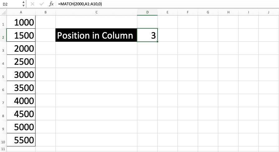
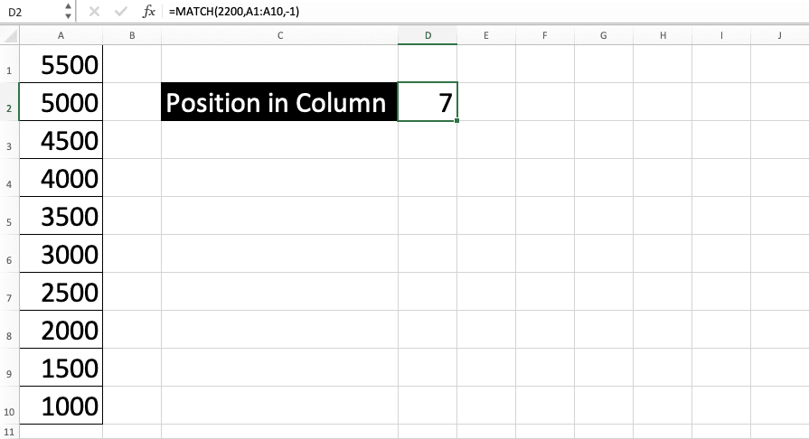
   • The example of the MATCH result with the 0 lookup method input
     
     
     
     
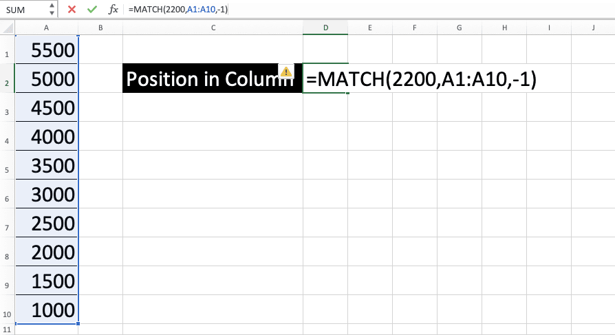
   • The example of the MATCH result with the -1 lookup method input
     
     
     
     
     
     
   • The example of the MATCH result with the 1 lookup method input
     
     
     
     
     
     

MATCH Formula Writing that Utilizes Wildcard Characters

What if the data you want to look for using MATCH has a part that can be filled with anything?

Maybe you just require the data to have a certain prefix or suffix. To do that requirement, you can use wildcard characters when inputting the data you want to look for in your MATCH.

There are 2 types of wildcard characters you can use in excel. They are:

• *: represents an unlimited number of characters that can be filled with any character
• ?: represents one character that can be filled with any character

As an example of the wildcard characters usage in MATCH, let’s say you input this for the data you look for.



With this input, MATCH will try to find the position of any data which has the prefix of “Da”. Data such as “Dart”, “Dazzle”, “Dash”, or other similar data can be the one that MATCH takes the position of. This is because you use the * symbol behind “Da”, which represents an unlimited number of any characters.



On the other hand, if you input like this in your MATCH.



Then, MATCH will lookup for data with a “Da” prefix, followed by one character of any kind. The data can be something like “Dai”, “Day”, “Das”, or other similar data.

However, the data cannot be something like “Dart”, “Dazzle”, “Dash”, or other data which have more than one character after “Da”. This is because you use a ? symbol, not *, behind your “Da” input, which represents one number of any character in excel.

As the implementation example of MATCH with these wildcard characters, take a look at the screenshot below.



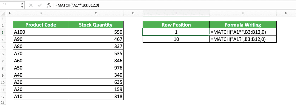
In the example, we can see the results of the wildcard characters implementation within MATCH. By using a * symbol in your data input (“A1*”), MATCH will take the position of any data with the “A1” prefix. In the example, MATCH takes the row position of “A100” data, which is 2.

Meanwhile, if we use ?, then MATCH will try to find data that has an “A1” prefix plus one more character. In the example, MATCH doesn’t take the row position of “A100” because this data has two characters after “A1”. Instead, MATCH takes the row position of “A10” data, which is 10. This is because only “A10” has only one more character after “A1”.

Another thing: If you want to use * and ? symbols in your MATCH input, then you must write a ~ symbol before (example: if you input “Da~?” in your MATCH, then it will try to find data with “Da?” as its value).

MATCH Formula that is Case-Sensitive in Its Lookup Process: MATCH TRUE EXACT

In its data position lookup process, MATCH doesn’t differentiate between capital and small letters. If, for example, the data you look for is “APPLE”, then if MATCH finds “apple”, it will produce that “apple” position.

What if we need to differentiate between capital and small letters in our data lookup position process? We can do that by combining MATCH with TRUE and another excel formula, EXACT.

Generally, here is the writing form of the combination to do the position lookup process of our data.



Notice the curly brackets around the formula? They are symbols that we use an array formula form. We must use this formula form because we input a cell range into EXACT, which normally accepts an individual data input.

To get an array formula form, you must press Ctrl + Shift + E buttons simultaneously after you finish writing your formula. Don’t press Enter like a normal formula because that will only make your formula produces an error.

The explanation of the process that happens in the formula is as follows. First, we use EXACT to match data in a case-sensitive way. The data matched is the data we want to look the position for and each data in our row/column.

Because we use EXACT like that, it will produce an array that contains TRUE and FALSE. Those TRUE/FALSE is for each data in our row/column. TRUE means the data is an exact match with the one we want to find the position for. FALSE means the data doesn’t match.

In the MATCH writing, we input TRUE as the data we want to lookup the position for. Because of that input, MATCH will look for the TRUE position in the TRUE FALSE array produced by EXACT. If it finds the position, then that means it has found our data position in a case-sensitive manner too!

Because of that, we will get the data position we look for while also considering the difference of capital and small letters!

Additionally, we use 0 for the lookup method input because the data we look for must be a text (because we need to consider its capital and small letters). If the lookup method input is -1 or 1, then we can get an error from our MATCH.

As an implementation and result example of this MATCH TRUE EXACT, look at the screenshot below.



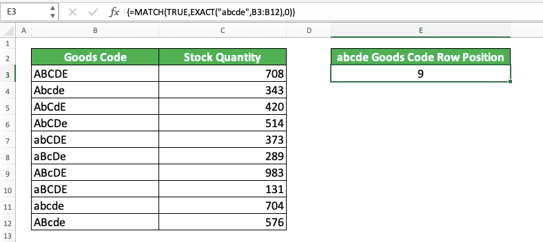
In the example, we can see how MATCH TRUE EXACT can lookup a data position in a case-sensitive manner. If we just use MATCH, then the result there will be 1.

This is because MATCH cannot differentiate between capital and small letters. Thus, it will think “ABCDE” is the same as the data we look for (“abcde”).

As an example of the array result from EXACT, we get an array result like this in the example above.



Each data that doesn’t exactly match with the data we look for, “abcde”, is FALSE while the matched one is TRUE. Because the data we look for in MATCH is TRUE, then it will get this TRUE position in the array.

In the example’s EXACT array result, TRUE is in the 9th position. Because of that, the formula produces 9, the same position with the “abcde” position in the code column!

Confirmation Whether There is a Specific Data in a Row/Column: IF ISNUMBER MATCH

What if we want to confirm whether there is specific data in a row/column? Can we use MATCH for that? The answer is we can and one of the ways to do it is combining our MATCH with IF and ISNUMBER.

The general writing form of IF, ISNUMBER, and MATCH combination to confirm data existence is as follows.



In the formula writing, we look for our data as usual using MATCH. After we get the result, we test it using ISNUMBER.

Because a MATCH result is always a number, if the data exists, then ISNUMBER will certainly produce TRUE. The TRUE from ISNUMBER will make our IF produces its TRUE result, which is “Yes”.



If MATCH cannot find the data, then it will produce an error and thus, ISNUMBER will certainly produce FALSE. This makes IF give the FALSE result we specify in it, which is “No”.

As an additional note, we must use 0 as the lookup method input because we need to find an exact match. If we use -1 or 1, then MATCH can find different data value if it doesn’t find the data we want. This can make our IF produces a wrong TRUE/FALSE result.

And, of course, we can use other words besides “Yes” and “No” for the IF result. It is up to you what words you think are the most suitable to confirm your data existence!

To understand better the use of IF ISNUMBER MATCH, here is its implementation example in excel.



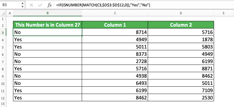
In the example, we check each data in column 1, whether it also exists in column 2. We check them using the combination of IF, ISNUMBER, and MATCH formulas.

In the MATCH input, we use $ symbols in the cell range so we can easily copy our formula to all rows. We input column 2’s cell range, with the data we look for is each data in column 1.

As for the TRUE and result inputs in the IF, we use the words “Yes” and “No”. This causes if MATCH finds the column 1 data we look for, then our formula will produce “Yes”. If not, then it will produce “No”.

By doing this IF ISNUMBER MATCH writing, we can confirm the existence of our data fast!

Formulas Combination for an Effective Data Lookup Process: INDEX MATCH

Often use VLOOKUP and/or HLOOKUP to look for your data in excel? If you understand how to use the INDEX MATCH combination, you might prefer to use it more than VLOOKUP/HLOOKUP!

Generally, the writing of the INDEX MATCH combination to look for data in excel is as follows.



In the INDEX MATCH combination, we use MATCH as the row and/or column position input of INDEX. As we know, INDEX can give us data from a cell range based on its row and column positions inputs. Because MATCH can give us data position in a row/column, we can combine them to look for our data effectively.

If we know the data row/column position in the cell range, then we can change MATCH with the position number. This makes INDEX MATCH very flexible in its implementation to do a data lookup process in excel.

As a simple example of INDEX MATCH implementation in excel, you can see the following screenshot.



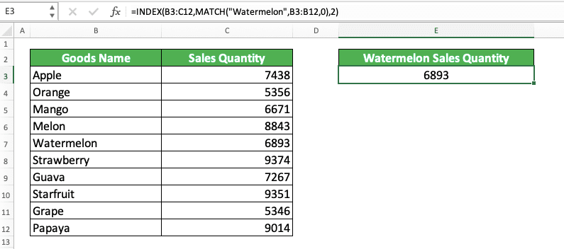
By using INDEX MATCH, we can get the watermelon sales quantity in the table on the left easily. Just specify the table’s cell range in INDEX and find the watermelon in the goods name column using MATCH.

We input 2 as the column position because we already know the sales quantity data is in the table’s second column. By giving our inputs correctly in the INDEX MATCH writing, we can immediately get the watermelon sales quantity we want!

If you want to learn further about INDEX MATCH, you can do it in our tutorial that specifically discusses it here.

Exercise

After you have learned completely about MATCH, now let’s do an exercise. This is so you can deepen your understanding on this formula’s implementation!

Download the exercise file and answer all the questions. Download the answer key file if you have done the exercise and want to check your answer. Or maybe when you are confused about how to answer the question!

Link to the exercise file:
Download here

Questions

1. What is the position of 177 in column B? If you cannot find the exact value, find the closest larger value position!
2. What is the position of 634 in column C? If you cannot find the exact value, find the closest smaller value position!
3. What is the position of 500 in column D? If you cannot find the exact value, find the closest smaller value position!

Link to the answer key file:
Download here

Additional Note

• The data position lookup process by MATCH is not case-sensitive
• If MATCH finds more than one matches, then it will take the most left/top match position
• There is a restriction for the number of characters in the data you look for. The upper limit is 255 characters

Related tutorials you will want to learn too: