How to Use the TRANSPOSE Formula in Excel: Functions, Examples, and Writing Steps

In this tutorial, you will learn how to use the TRANSPOSE formula in excel completely.

When working in excel, we sometimes need to flip over a data table for various purposes. We want its horizontal parts become vertical and its vertical parts become horizontal. One of the easiest ways to do this flipping process in excel is by using the TRANSPOSE formula.

Want to know more about TRANSPOSE and how to use the formula properly in excel? Read this tutorial until its last part!

Disclaimer: This post may contain affiliate links from which we earn commission from qualifying purchases/actions at no additional cost for you. Learn more

Want to work faster and easier in Excel? Install and use Excel add-ins! Read this article to know the best Excel add-ins to use according to us!

What is the TRANSPOSE Formula in Excel?

TRANSPOSE is an excel formula that helps us to flip a cell range over. This means that it will make the cell range vertical parts to horizontal and its horizontal parts to vertical.

TRANSPOSE Function in Excel

You can use TRANSPOSE to help you turn around a cell range easily in excel.

TRANSPOSE Result

The TRANSPOSE result is a cell range that is the opposite in orientation to the cell range you input into it.

Excel Version from Which We Can Start Using TRANSPOSE

We can start using TRANSPOSE in excel since excel 2003.

The Way to Write It and Its Input

Here is the general writing form of TRANSPOSE in excel



Just input the cell range you want to turn over the orientation of to TRANSPOSE. As the result we expect from TRANSPOSE is an array (cell range), we should use the excel array formula form. This is why we have curly brackets around our TRANSPOSE formula writing.

We turn TRANSPOSE into an array formula by pressing Ctrl + Shift + Enter buttons after we write the formula. We should also highlight the cell range where we want to put its result first to get the result correctly.

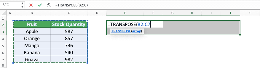
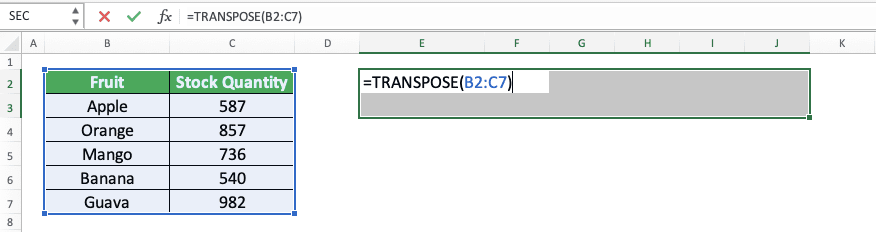
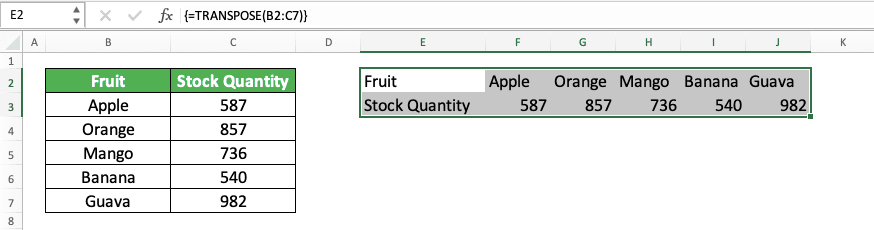
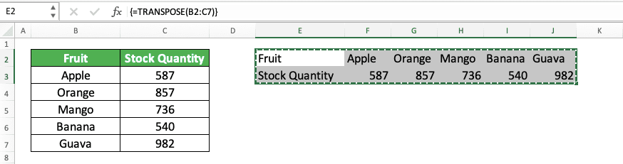
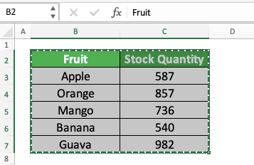
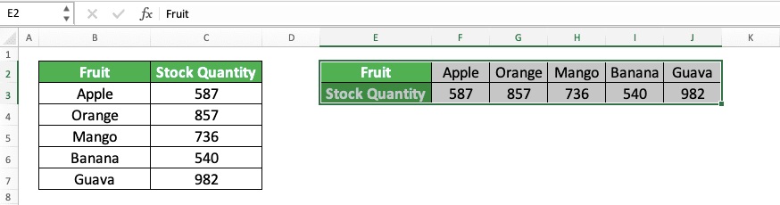
Example of Its Usage and Result

Here is an implementation example of TRANSPOSE in excel.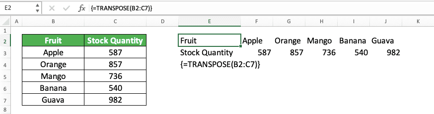



In the example, you can see the result and how we write the TRANSPOSE formula in excel.

When we write TRANSPOSE, we just need to input the cell range we want to change the orientation of. Remember to highlight the result cell range and press Ctrl + Shift + Enter after the formula writing to get the result correctly.

As you can see in the example result, TRANSPOSE doesn’t carry over cell formatting in its result. It only produces the value of the cell range you input in the opposite orientation.

Writing Steps

After we have discussed the TRANSPOSE writing form, input, and implementation example, now let’s discuss its writing steps. As it only needs only one simple input, the writing steps should not be too hard to follow.

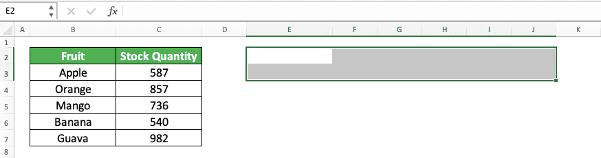
1. Highlight the cell range where you want to put your TRANSPOSE result. The cell range number of rows must be the same as the number of columns of your TRANSPOSE cell range input. The cell range number of columns must be the same as the number of rows of your TRANSPOSE cell range input
   
   
   
   
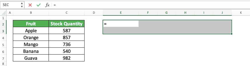
2. Type an equal sign ( = )
   
   
   
   
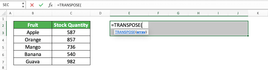
3. Type TRANSPOSE (can be with large and small letters) and an open bracket sign after =
   
   
   
   
4. Input the cell range which orientation you want to turn over (vertical to horizontal or horizontal to vertical)
   
   
   
   
5. Type a close bracket sign
   
   
   
   
6. Press Ctrl + Shift + Enter buttons
7. Done!
   
   
   
   

Transpose Without Zeroes for Blanks: TRANSPOSE IF

If we have blank cells in the cell range we input to TRANSPOSE, we will get zeroes in our TRANSPOSE result.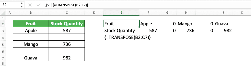



What if we just want to keep the blank cells blank in our TRANSPOSE result? Well, for that, we can combine our TRANSPOSE formula with an IF.



Here is the general writing form of the two formulas combination for the purpose.



Quite simple, isn’t it? We just have to make a logic condition for the blank cells in the IF we write in our TRANSPOSE.

If the cells in the cell range are blank, then we want to keep it blank. We declare this in our IF by inputting the logic condition where the cell range is equal to a blank (the symbol for the blank in excel is empty quotes ( “” )). We input a blank too as the IF true result to say that we want to keep the blank cells blank.

For the IF false result, we input the cell range itself. That is to say that we want to keep the cells’ content as they are if they are not blank.

After we write an IF like that in our TRANSPOSE, we press Ctrl + Shift + Enter and we will get our result! Don’t forget to highlight the result cell range first so we can get our TRANSPOSE IF result in full.

Here is the implementation example of the TRANSPOSE and IF formulas combination in excel.



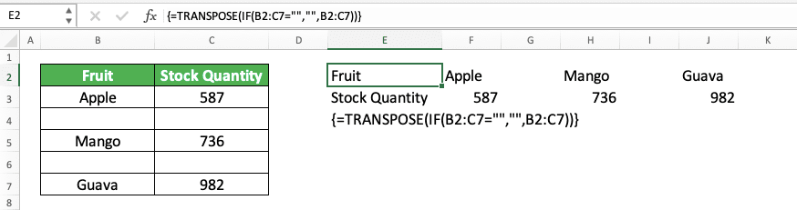
As you can see there, we manage to keep the blank cells blank in our TRANSPOSE result. That is because we combine our TRANSPOSE and IF formulas in the way that we have discussed before!

Get a Static Transpose Result 1: Paste Value

If you use TRANSPOSE to transpose your cell range, you will get a dynamic result. That means when you change the content of the cell range you input into TRANSPOSE, your TRANSPOSE result will change too.

What if you want a static result that isn’t going to change whatever you do to your transpose source, instead? One way to get a static transpose result is to paste value your TRANSPOSE formula writing.

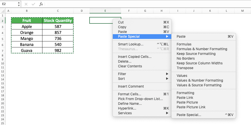
The way to paste value that is quite easy. First, highlight the cell range which is the result of your TRANSPOSE formula. Then, press the Ctrl + C buttons so the cell range goes into a copy mode like this.



Then, you can just right-click on the cell range and highlight Paste Special in the choices that show up. After that, choose Paste Value.



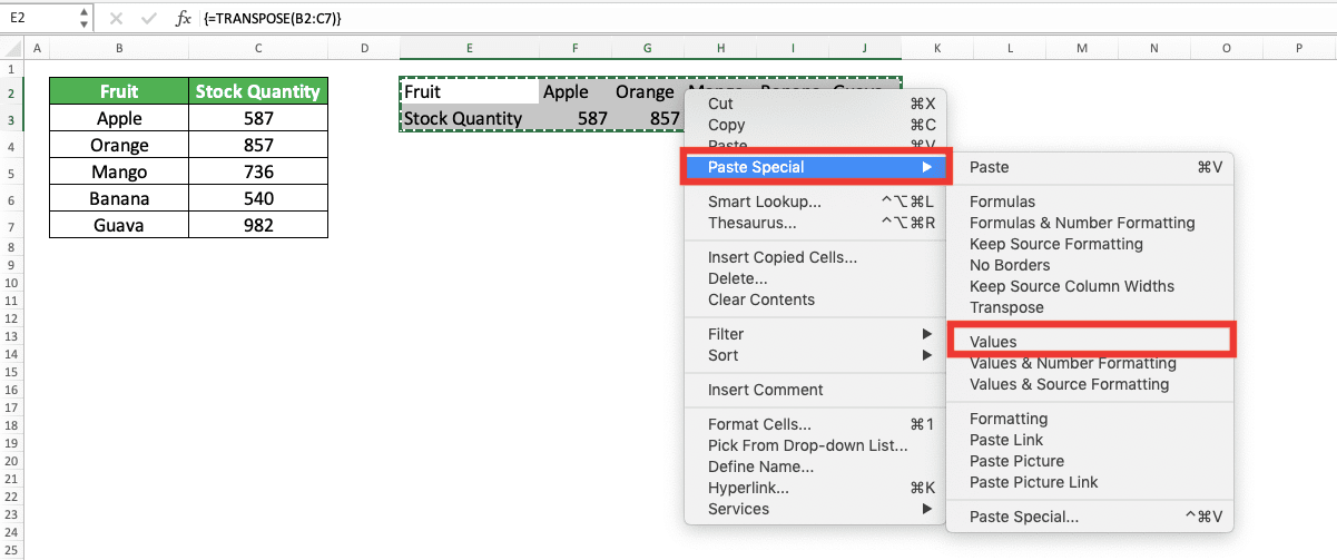
Press the Esc button on your keyboard to remove the copy mode from your cell range.

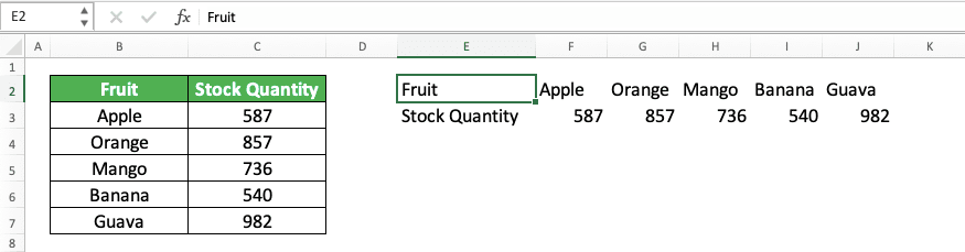
By doing those steps, you have pasted value your TRANSPOSE formula writing! That means you have removed the TRANSPOSE formula writing and just keep its result. The cell range from the transpose process should be static now as a result.

Get a Static Transpose Result 2: Paste Transpose

Another way to get a static transpose result, without involving TRANSPOSE, is by using paste transpose. Similar to paste value, paste transpose is also a part of paste special feature in excel.



To paste transpose, first, highlight the cell range you want to transpose. Then, press the Ctrl + C buttons so the cell range will be in a copy mode like this.



Then, select the most top-left cell where you want to put your transposed result. After that, right-click on the cell, highlight Paste Special, and choose Transpose.



Press the Esc button to remove the copy mode from your cell range.

By doing that, you have transposed your cell range and the result will be static! Unlike TRANSPOSE, paste transpose will copy the cell range formatting too with its values.

Exercise

After you have learned how to use TRANSPOSE in excel completely, let’s do an exercise to deepen your understanding!

Download the exercise file and do all the instructions below. Download the answer key file if you have done the exercise and want to check your answers!

Link to the exercise file:
Download here

Instructions

Give your answer on the appropriate cells for each instruction number in the exercise file!

1. Transpose cell range no. 1 with the TRANSPOSE formula!
2. Transpose cell range no. 2 by combining the TRANSPOSE and IF formulas! Then, paste value the result!
3. Transpose cell range no. 3 by using paste transpose!

Link to the answer key file:
Download here

Additional Note

If you want to delete a TRANSPOSE result, then you should delete all of them. That is because excel treats the result with the TRANSPOSE formula writing as one entity that we cannot separate.

However, if you have pasted value the result, then you can delete it one by one.



Related tutorials you should learn from: