AVERAGE Formula in Excel: Functions, Examples, and How to Use

In this tutorial, you will learn everything you need to know about the implementation of the AVERAGE formula in excel.

Average is a calculation process we often need to do when we want one number to represent a group of numbers. If you process your numbers in excel, then the software provides the AVERAGE formula to help us calculate an average fast.

Want to master AVERAGE so you can optimize your numbers processing in excel? Read this tutorial until its last part!

Disclaimer: This post may contain affiliate links from which we earn commission from qualifying purchases/actions at no additional cost for you. Learn more

Want to work faster and easier in Excel? Install and use Excel add-ins! Read this article to know the best Excel add-ins to use according to us!

What is AVERAGE in Excel?

We can define AVERAGE as a formula that can average numbers that we have in excel fast and accurately.

AVERAGE Function in Excel

AVERAGE can help us to get the average of a group of numbers in excel.

AVERAGE Result

An AVERAGE result is a number that represents the average of the numbers we give as inputs to this formula.

Excel Version from Which We Can Use AVERAGE

We can use the AVERAGE formula in excel since excel 2003.

The Way to Write it and Its Inputs

Here is the general writing form of AVERAGE in excel.



The only input you need to give to AVERAGE is the numbers you want to average. You can input those numbers by typing them directly in AVERAGE or by referring to cell coordinates or cell ranges.

Usually, we only input one cell range to AVERAGE which contains all the numbers we want to average. If you happen to give more than one inputs, then don’t forget to separate them with commas ( , ).

Example of Its Usage and Result

Here is the implementation example of AVERAGE in excel. You can see the real writing and result of the formula here too.



In this example, we have a full year sales quantity data and we want to get the average of the numbers. To calculate it fast, we use the AVERAGE formula in excel.

Just input the cell range containing the sales quantity numbers (sales quantity column cell range) and press enter. AVERAGE will immediately give its average calculation result for us!

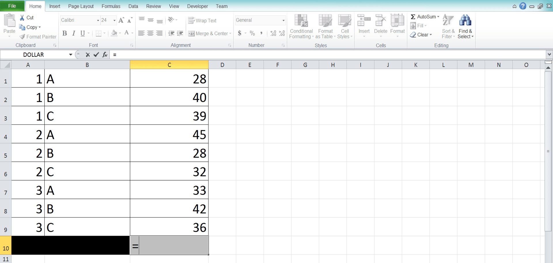
Writing Steps

After you have seen the writing form, inputs, and implementation example of AVERAGE, let’s learn its writing steps. They are quite simple to follow as you can see in the following.

1. Type an equal sign ( = ) in the cell where you want to put the average number
   
   
   
   
2. Type AVERAGE (can be with large and small letters) and an open bracket sign after =
   
   
   
   
3. Input all the numbers you want to average by directly typing them or through cell or cell range coordinates. If you give more than one input, separate them with comma signs
   
   
   
   
4. Type a close bracket sign after you have inputted all the numbers you want to average
   
   
   
   
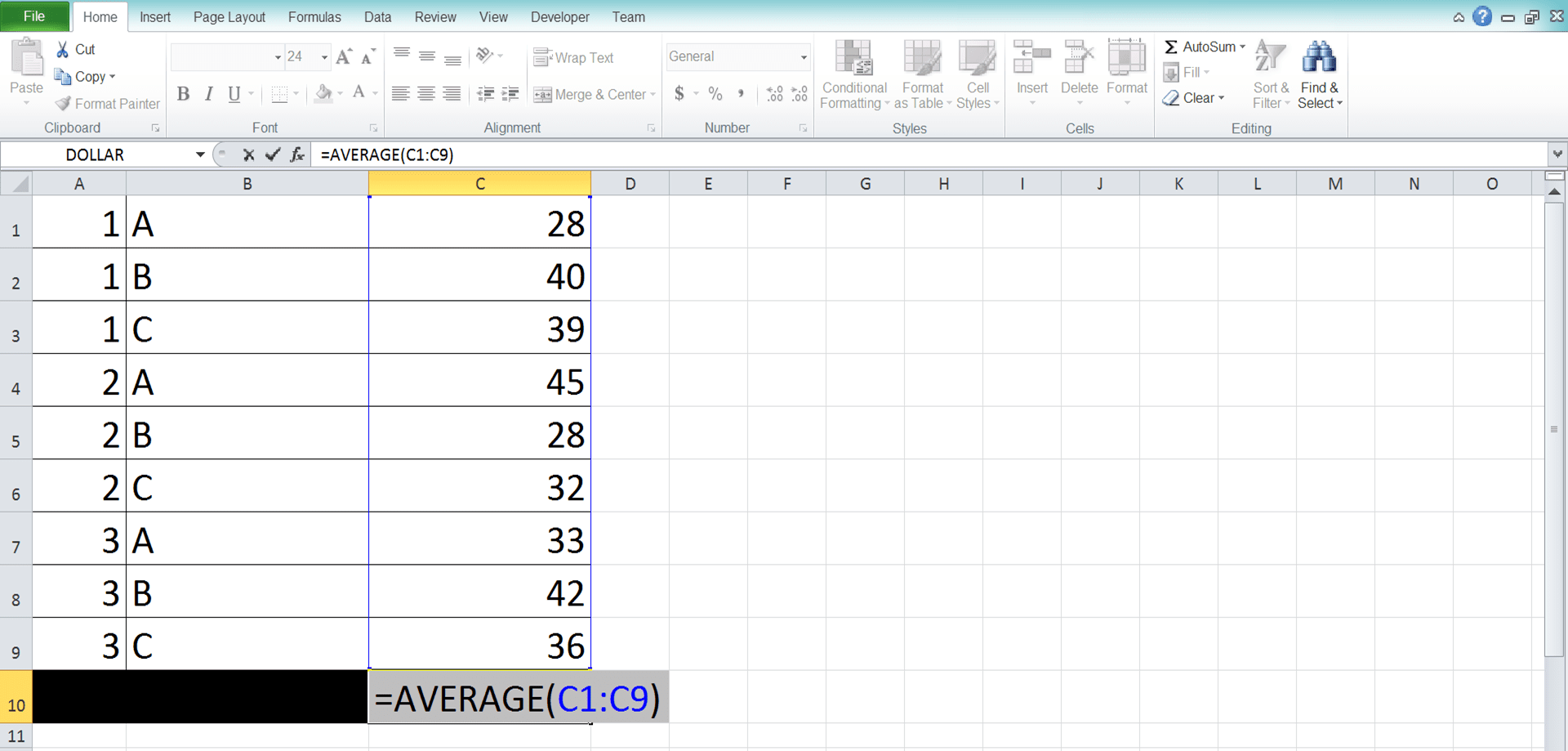
5. Press Enter
6. Done!
   
   
   
   

AVERAGE that Involves Logic Values and Text: AVERAGEA

Need to somehow involve text and logic values in your average calculation in excel? If that is what you want, then you shouldn’t use AVERAGE as your go-to formula. You should use AVERAGEA instead.

AVERAGEA will average your numbers, texts, and logic values in its calculation. AVERAGEA will assume TRUE logic value as 1 and text and FALSE logic value as 0.



The writing form of AVERAGEA in excel is quite similar to AVERAGE as you can see in the following.



And here is the AVERAGEA implementation example in excel.



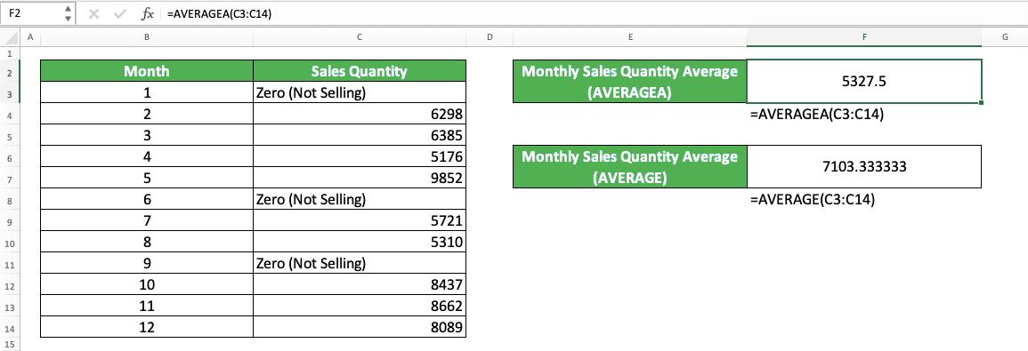
In the example, we have a data set that we average using AVERAGE and AVERAGEA. You can see the writing form and result from both formulas and their differences too.

In the data set, we have three texts which tell us there are no sales in that month. When we calculate the average of this data set, AVERAGE ignores them and thus, only averages nine numbers there. Meanwhile, AVERAGEA considers the three texts as 0 and average 12 numbers as a result.

Because of that, the results from AVERAGE and AVERAGEA are different in the screenshot example. If there is no text (and logic values) in the input of both, then their results should be similar.

AVERAGE with Criteria (AVERAGE IF): AVERAGEIF/AVERAGEIFS

Need to average only the numbers from the data entries that fulfill your criteria? You can use AVERAGEIF/AVERAGEIFS to help you instead of AVERAGE.

You can use AVERAGEIF if you only have one criterion and AVERAGEIFS if you have one or more criteria. The general writing forms for both in excel are as follows.

AVERAGEIF



AVERAGEIFS



In AVERAGEIF, you only need to input one pair of data range and criterion as it can only accept one criterion. The criterion will evaluate all data in the data range. After that, AVERAGEIF will average the numbers in the number range which are parallel with the data that fulfill the criterion.

The number range input in AVERAGEIF is optional. If you only input the data range, then AVERAGEIF will average the numbers there (that fulfill your criterion).

In AVERAGEIFS, you input the number range first before the data range and criterion pairings and this isn’t optional. For the data range and criterion pairings, you can input one or more pairs. The criterion you input will only evaluate the data in the data range we input before it.

For the AVERAGEIF and AVERAGEIFS inputs, the data ranges and number range should have the same size and parallel in position. This is so it will be easier for us to check their results if we need to.

Here is the implementation example of AVERAGEIF and AVERAGEIFS in excel.



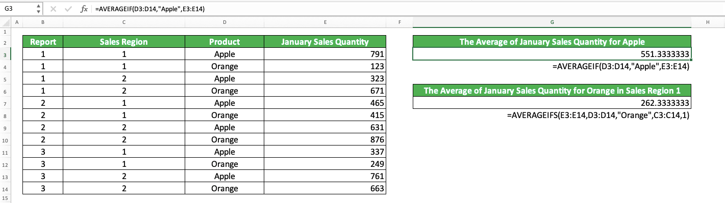
We have a data set with several columns here, including the January sales quantity column which contains sales quantity numbers. We want to calculate two averages of the January sales quantity, for apple and for orange in sales region 1.

For the apple criterion, we can use AVERAGEIF since it only has one criterion. Just input the January sales quantity column, product column, and the “apple” criterion.

For the orange in sales region 1 criterion, we should use AVERAGEIFS since there are two criteria there. We input the January sales quantity column, the product column and its criterion (orange), and the sales region column and its criterion (1).

Use them correctly and we can get our numbers average based on the criteria we have!

The AVERAGE Usage in a Filtered Data: SUBTOTAL

SUBTOTAL is a formula that specializes itself in processing cell range data where we apply a filter on. We can utilize several excel formulas to the filtered cell range through SUBTOTAL. One of them is AVERAGE.

Why don’t we use AVERAGE directly to the filtered cell range instead of using SUBTOTAL?

If we use AVERAGE, then it will involve the numbers that our filter hides too. When we just want to get the average of the numbers that pass our filter, we should use SUBTOTAL instead.

Here is the general writing form of SUBTOTAL to apply AVERAGE in a filtered cell range.



The 1 or 101 input there is the AVERAGE code input for SUBTOTAL. Input 1 if you also want to calculate the numbers in the cells you hide manually in the filtered range. If you want to ignore them instead, then input 101.

After inputting the AVERAGE code, you can input the filtered range you want to calculate the average of the numbers of. You can input more than one filtered range although people mostly input just one filtered range.

To better understand the AVERAGE implementation through SUBTOTAL in excel, here is an example.



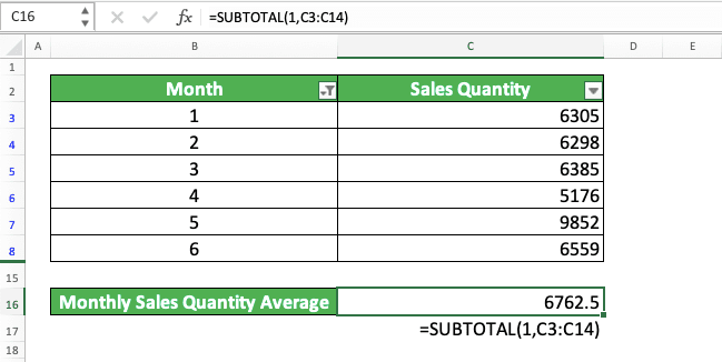
In this example, again, we have a monthly sales quantity data set.

We have filtered the data set cell range so it only shows us the sales quantity from month 1 to 6. If we want to apply AVERAGE to the sales quantities from that filtered cell range, then we should use SUBTOTAL.

We input the code of 1 and the filtered cell range to our SUBTOTAL. We can either input 1 or 101 here since we don’t have manually hidden cells in the filtered cell range. The filtered cell range we input is the sales quantity column which we have filtered.

Write your SUBTOTAL correctly and you will immediately get the average of the numbers in your filtered cell range! Just like what you see in the example above.

AVERAGE Largest/Smallest Values: AVERAGE LARGE/SMALL

Need to average only the largest/smallest numbers from a group of numbers you have in excel? You can use AVERAGE to do this calculation. However, if you want to do it in one writing, then you should combine the formula with LARGE (for the largest numbers)/SMALL (for the smallest numbers).

The general writing form of the AVERAGE and LARGE/SMALL combination in excel is as follows.



We write the LARGE/SMALL formula in our AVERAGE for this combination. In the LARGE/SMALL, we input the cell range where our group of numbers is. We also input an array containing the ascending (SMALL)/descending (LARGE) orders of the numbers we want to average.

For the array input example, let’s say we want to average the first to sixth-largest numbers. To get that average, we should input this array to our LARGE formula: { 1 , 2 , 3 , 4 , 5, 6 }.

If you have used LARGE/SMALL before, then you may know that both formulas usually only process one number. Thus, its second input should only contain one descending/ascending order to produce the largest/smallest number we want.

However, if we input a number array to the formula, then we can get an array containing several numbers too. This fact is what we utilize in this AVERAGE and LARGE/SMALL combination. By using the fact, we can average the largest/smallest numbers in one formula writing!

You can see the implementation example of the formulas’ combination in the screenshot below.



We use the data set we have used for the AVERAGE implementation example earlier in this tutorial. Now, we want to calculate the average of the three largest and smallest monthly sales quantities. We can use the combination of AVERAGE and LARGE/SMALL to make the calculation process much easier and faster.

We input the sales quantity column cell range into our LARGE and SMALL in each formula writing. Then, we input a { 1 , 2 , 3 } array too so we can average the first, second, and third-largest/smallest numbers.

We do all those LARGE/SMALL formula writings in our AVERAGE. As a result, we get the average of the three largest/smallest monthly sales quantities that we want!

AVERAGE to Calculate the Moving Average

By using AVERAGE, you can also calculate the moving average in excel. However, you need to place your data chronologically in sequence so the formula writing process can be easier.

There are two ways to calculate the moving average: by using AVERAGE only or by combining AVERAGE, OFFSET, MIN, and ROW. The AVERAGE, OFFSET, MIN, and ROW combination can give you much more flexibility in terms of the moving average calculation period.

To calculate the moving average in excel by only using AVERAGE, here is the general writing form.

The cell range coordinate in the AVERAGE formula should be relative (no dollar symbols in the cell range coordinate). That way, we can copy it easily to get all our moving average results. The size of the cell range we input depends on the period length we calculate in our moving average.

Meanwhile, the writing form of the AVERAGE, OFFSET, MIN, and ROW combination for the excel moving average calculation is as follows.



In the formula writing, OFFSET will make your cell range moves along with your moving average calculation location. You can also change the period length of your moving average easily. Just change the period_length input in the MIN formula inside the OFFSET.

We use MIN and ROW combinations so we can calculate the moving average too if the period length is long. Sometimes, the period length can be longer than what OFFSET can stretch for our top numbers. The MIN formula there will control so our OFFSET won’t stretch beyond our numbers range.

To do that, our MIN gets the smaller number between our period length and our ROWs subtraction result. The ROWs we subtract are ROW for the cell where we write our formula (thus we don’t give any input to this ROW) and ROW for our top number cell. We add 1 to the ROWs subtraction result to make it produce the right number.

We also add the minus symbol before the MIN because we want OFFSET to stretch up. That is because the moving average calculation takes the period numbers before the period we calculate.

The formula writing form above assumes your numbers sequence is in rows (the most common form). If it is in columns, then you should swap the MIN formula and 1 inputs position. As we need to copy the formula to calculate our moving averages, make the number cell reference in the OFFSET relative.

To make you understand better about the moving average calculation using just AVERAGE, here is its implementation example.



As you can see, we calculate the sales quantities moving average for 3 months period there using AVERAGE. Just write AVERAGE that calculates the top number moving average and copy it down to get all our moving average results. As AVERAGE ignores non-numbers in its average calculation, we shouldn’t have problems getting the top number moving average.

However, it can be troublesome if we need to change the period to 5 or 6 months. That is because we need to rewrite all of our AVERAGE formulas to do that.

Moreover, your period length can be larger than what you can input for your first moving average. That makes you need to write separate AVERAGE formulas for the top numbers so you can get all the moving averages.

If you have similar problems to what we just discussed, then you can combine AVERAGE, OFFSET, MIN, and ROW instead. The implementation example of the formulas’ combination is as follows.



Here, you can see the real writing and result example of AVERAGE, OFFSET, MIN, and ROW combination to calculate moving averages. We write them using the pattern we have just discussed. As the moving average period there is 3 also, the results are the same with our AVERAGE only method earlier.

However, one advantage of using these formulas combination is the easiness to change the moving average period. We just change the E3 cell value we refer to in our formula writing there and the period will change.



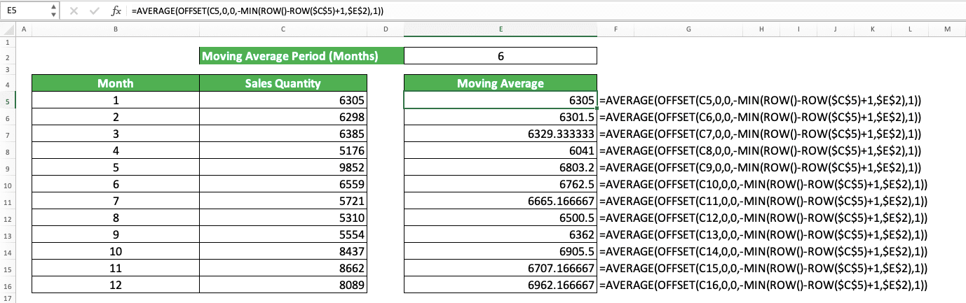
If we don’t use MIN and ROW as our OFFSET input there, then our first few formulas will produce errors. That is because the six months length is greater than what our first few OFFSET formulas can stretch up to.

Shortcut for AVERAGE in Excel: AutoAverage

There is a feature you can use to shortcut your AVERAGE formula writing for a number sequence. That feature is AutoAverage, one of the variants in the AutoSum feature.

The way to activate the AutoAverage feature in excel is quite easy. You can follow the steps below that we also illustrate using some screenshots.

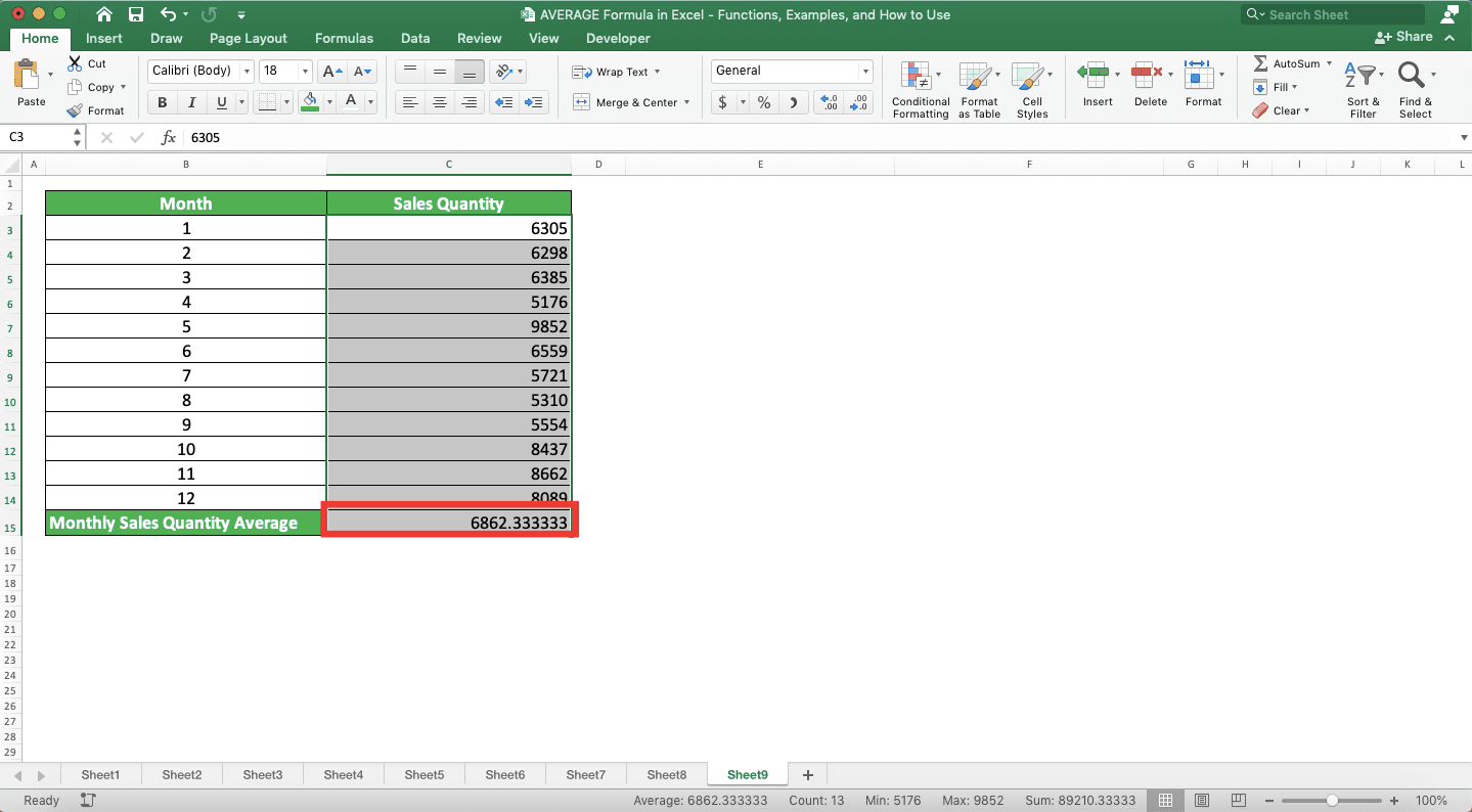
First, highlight the number sequence cell range you want to average or put your cell cursor just outside the cell range.



Then, go to the Home or Formulas tab in your excel workbook. Click the AutoSum button dropdown there and choose Average.

AutoAverage choice in the Home tab



AutoAverage choice in the Formulas tab



Excel will automatically write an AVERAGE with your number sequence cell range input for you. As a result, you will immediately get your number sequence average result!



Easy to do, isn’t it?

Exercise

After you learned how to use the AVERAGE formula in excel, let’s do an exercise. This is so you can practice what you have just learned and understand the lessons better.

Download the exercise from the following link and answer the questions below. Download the answer key file if you have done the exercise and sure about the result!

Link to the exercise file:
Download here

Questions

1. What is the average of B1 to B10 numbers?
2. What is the average of C1 to C10 numbers?
3. What is the average of D1 to D10 numbers?

Link to the answer key file:
Download here

Additional Note

You can give up to 255 different inputs in an AVERAGE formula.



Related tutorials you should learn: